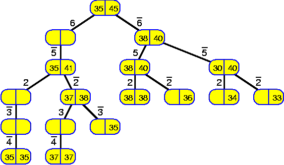
For each chapter an estimated duration is given. This is just an indication. Inside the chapters particularly important ideas and short key notes are highlighted without introductory text. There are many pictures. They are intended to be self-explaining. Mostly there is no direct reference to them in the text.
In the course of the lecture we will encounter the following data structures:
Algorithms can be formulated in many ways. Consider the problem of finding the maximum from a set of n numbers which is stored in an array a[]. The algorithm can be formulated as follows:
Start by initializing a variable, which we will call M here after, with the value of a[0]. Then check the numbers a[i] starting from a[1] and going all the way to a[n - 1] in this order. Each of these numbers is compared with the current value of M, and if a[i] happens to be larger than M, then a[i] is assigned to M.This is definitely an algorithm. All the important details are mentioned. This is about how a (good) cooking recipe might be given or how one may be instructed to repair a punctured tire.
However, in computer science texts, it is common to use a slightly more formalized way of expression, using pseudo-code. Pseudo-code intermixes common program-language-like fragments with fragments in natural language. This is convenient, because this allows to express loops and tests more clearly. On the other hand, there is no need to declare variables. So, we might also write:
  function maximum(array a[] of length n)
    begin
      if (n equal to 0) then
        return some special value or generate an exception
      else
        M = a[0];
        for (all i from 1 to n - 1) do
          if (a[i] > M) then
            M = a[i];
        return M;
      fi;
    end.
In such a more formal notation one might also more easily detect that we
should also handle the case of an empty set correctly. In this simple case, we
could just as well have written C or Java code, but in general this may distract
from the essentials of the algorithm.
Actually all these notions should be written with the "element-of symbol", so one should say "T(n) = 6 * n^2 + 2 * n^3 + 345 is an element of O(n^3)", but it is very common to use the equality symbol. Nevertheless one should not be fooled by this: T(n) = O(f(n)) does not imply that O(f(n)) = T(n) (this is not even defined) or that f(n) = O(T(n)) (which might be true, but which does not need to be true).
By far the most common of these symbols is O(). This symbols gives us an upper-bound on the rate of growth of a function, allowing us to make an overestimate. In the chapter on union-find we will give an analysis of the time consumption and we will conclude that certain operations can be performed very efficiently, stating T(n) = O(f(n)) for some function f() which is almost constant. However, the actual result is even sharper, even in an asymptotic sense. Most other algorithms and data structures we study in this lecture are so simple that the time consumption of operations can be specified exactly. In that case we might even write T(n) = Theta(f(n)), but because it is typically the upper bound which interests us most, we will even in these cases mostly use O().
It is easy to show, just arguing formally, that if T_1(n) = O(f_1(n)) and T_2(n) = O(f_2(n)), that then T_1(n) + T_2(n) = max{O(f_1(n)), O(f_2(n))}. As an example we will prove this. All other relations in the book can be proven similarly. We know T_1(n) < c_1 * f_1(n) for all n > n_1, and T_2(n) < c_2 * f_2(n) for all n > n_2. This implies T_1(n) + T_2(n) < (c_1 + c_2) * max{f_1(n), f_2(n)}, for all n > max{n_1, n_2}.
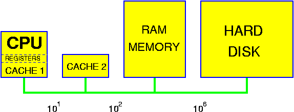
One should be aware that this model is only a coarse approximation of the reality that holds for modern computer systems. Of course, at least in theory, this is dealt with by the O() assumption: all operations are constant time, but the constants may be quite considerable. The most important aspect is the non-uniform cost of memory access. The following picture gives a very high-level view of a modern computer system.

Other factors may, however, be equally important. The main other factor is space. There are examples of problems that can be solved faster if we are willing to use more space. So, in that case we find a space-time trade-off. A trivial (but extreme) example is to create a dictionary for all words of at most five letters with 27^5 storage. After initialization, we can perform insertions, deletions and look-ups in constant time. Actually, applying the idea of virtual initialization (treated in one of the later chapters), the prohibitively expensive initialization does not need to be performed.
A further point that should be stressed here, is that when evaluating the performance of an algorithm, we consider the time the algorithm might take for the worst of all inputs. That is, we perform a worst-case analysis. Thus, if we state "this sorting algorithm runs in O(n * log n)", we mean that the running time is bounded by O(n * log n) for all inputs of size n. If on the other hand we say "this sorting algorithm has quadratic running time", we do not mean that it takes c * n^2 time for all inputs of size n, but that there are inputs (maybe not even for all values of n) for which the algorithm takes at least c * n^2 time for some constant c. This type of analysis is by far the most common in the study of algorithms, but occasionally one gets the feeling that this does not reflect the "real" behavior in practice. Maybe there only some rare very artificial instances for which the algorithm is slow. In that case one may also perform some kind of average case analysis. The problem is to define what the average case is. For example, when sorting n numbers, can one assume that all n! arrangements are equally frequent? In the real practice there may be a tendency to have some kind of clustering. The strong point of a worst-case analysis is that it leaves no room for such discussions. Furthermore, one can easily find many contexts, where one wants guaranteed performance.
Mathematics from several branches is needed. The following topics are of central importance in algorithmics: more
The mathematics in this lecture will mostly be of the elementary type, but we will also encounter a little bit of probability theory and we will deal with graphs, but not in a very theoretical way.
What does proving something by induction mean?
We now apply this proof method to the formula above. First we notice that sum_{i = 0}^0 a^i = 1 = (1 - a^{0 + 1}) / (1 - a). This gives our base case. Now assume that we have proven the equality for some arbitrary n >= 0. Then we can write
  sum_{i = 0}^{n + 1} a^i               =def of sum=
  sum_{i = 0}^n a^i + a^{n + 1}         =induction hypothesis=
  (1 - a^{n + 1}) / (1 - a) + a^{n + 1} =computation=
  (1 - a^{n + 2}) / (1 - a).
So, using the claimed property for n, we have proven it for n + 1.
Together with the basis, the axiom of proving by induction now allows to
conclude that the property holds for all n >= 0.
In a similar way many more of these relations can be proven. Often one needs a small twist that is not entirely obvious. For example,
The above arguments suggest that f(n) i ~= 1/2 * n^2. What is the exact value? A reasonable guess is that f(n) == g(n) for some polynomial of degree two g(n) = 1/2 * n^2 + b * n + c. We know that f(0) = 0 and that f(1) = 1. So, if f(n) == g(n), then we must have g(n) = 1/2 * n^2 + 1/2 * n + 0 = 1/2 * n * (n + 1). Notice that we do not yet claim that this is true: we have only explained how one can guess an expression and assuming its correctness determine the occurring parameters. Proving that indeed f(n) == g(n) for all n can be done with induction. The base case, n == 0, is ok because f(0) == sum_0^0 0 == 0 == 1/2 * 0 * (0 + 1) == g(0). So, assume f(n) == g(n) for some n >= 0 and all smaller values, then the following completes the proof:
   f(n + 1)                    =def of f=
   sum_{i = 0}^{n + 1} i       =def of sum=
   sum_{i = 0}^n i + (n + 1)   =induction hypothesis=
   1/2 * n * (n + 1) + (n + 1) =computation=
   1/2 * (n + 1) * (n + 2)     =def of g=
   g(n + 1).
More generally, you should know that similar formulas exist for f_k(n) = sum_{i = 0}^n i^k, for all finite k. Again approximating the sum by an integral, we find f_k(n) ~= n^{k + 1} / (k + 1). Guessing that this constitutes the leading term in a polynomial of degree k + 1, the expression can be derived: in general, a polynomial of degree d is uniquely determined when we know its value in d + 1 points: using these values, the coefficients can be determined by solving a system with d + 1 unknowns and d + 1 equations. For f_k we can take the values f_k(0), ..., f_k(k).
0! = 1,
n! = n * (n - 1)!, for all n > 0.
The general idea of a recursive definition of a function f is that
Clearly there is a problem here: one should assure that for all values n, the recursion terminates. That is, one should make sure that expanding the recursion, going from f(n) to f(n') to f(n''), ..., one ultimately reaches one of the base cases.
Not only functions can be recursive, but also programs and algorithms (in the light of the existence functional programming this is not surprising). In a recursive algorithm, it is fixed how some special cases can be treated and for all other cases it is told how they can be solved, using the solution of some other cases. As for recursive functions, the problem is to assure that for any possible input ultimately a base case is reached. That is, one should make sure that for any finite input the computation reaches one of the base cases in a finite number of steps and thus terminates.
A problem which can very well be solved in a recursive way is sorting. The task is to design an algorithm that sorts sets of numbers. Let n denote the cardinality (the number of elements) of the set to sort. As base case we take n == 1. In that case the algorithm simply outputs the single element, constituting a sorted set of size 1. For any n > 1, it performs the following steps:
The correctness of recursive algorithms is proven by induction. Mostly this is an induction over the size of the input. This works in the case of our sorting algorithm: for sets of size 1 the correctness is obvious. This is the basis of our inductive proof. So, let us assume the algorithm is correct for all sets of size n and smaller, for some n >= 1. Consider a set of size n + 1. The algorithm splits this set in S_0, S_1 and S_2. S_0 and S_2 have size at most n, and thus we may assume by the induction hypothesis, that they are correctly sorted. But then the whole algorithm is correct, because all values in S_0 are strictly smaller than all those in S_1, which in turn are strictly smaller than all those in S_2.
As an example we consider the time consumption of the recursive sorting algorithm presented above. We can estimate
T(n) == T(n_0) + T(n_2) + c * n,for some constant c, where n_0 = |S_0| and n_2 = |S_2|. The reason behind this estimate, is that splitting a set as specified can somehow be performed by considering all elements once and then putting them in the right bag. In any reasonable implementation, this takes linear time, covered by the term c * n. Sorting S_0 takes T(n_0) and sorting S_2 takes T(n_2). As long as we do not spend too long on selecting x, all other operations take constant or at most linear time.
In this case the problem is that we do not know the values of n_0 and n_2, because these depend on the selected item x. The only thing we know is that n_0 + n_2 <= n - 1. In a later chapter this algorithm is considered again. Here we will only analyze its worst-case. The worst that can happen, is that we split the set very unevenly, for example by selecting the largest element. In that case n_0 == n - 1 and n_2 == 0. If this unlucky situation happens again and again, then the time consumption is given by the following recurrence relation:
T(1) = c,Here c is chosen so large that the expressions on the right actually give an upper bound on the time consumptions on the left. Expanding the recurrence relation several steps, one soon discovers that T(n) == f(n) for f(n) == sum_{i = 1}^n (c * i).
T(n) = T(n - 1) + c * n, for all n > 1.
The formal proof that T(n) == f(n) goes induction. The basis of the induction is given by T(1) = c = f(1). Assuming that T(n) == f(n) for some value n and all smaller values, it follows that
  T(n + 1)           =def of T()=
  T(n) + c * (n + 1) =induction assumption=
  f(n) + c * (n + 1) =def of f(n)=
  f(n + 1).
But now we can use our knowledge on the sum of a arithmetic progression to conclude that for this function T(), T(n) = c/2 * n * (n + 1) = Theta(n^2).
As soon as one believes to know the solution of a recurrence relation, it is normally not hard to verify the correctness of this believe. However, in general, it may be very hard to find such solutions. There are mathematical methods which allow to solve several classes of common recurrence relations. Here we will not discuss these methods (which are similar to solving differential equations). Rather we list some of the most common types for reference purposes. We also indicate some of the algorithms whose time consumption is described by them:
| T(n) <= T(alpha * n) + c | T(n) <= c * log_{1/alpha} n, for alpha < 1 | binary search, Euclidean algorithm |
| T(n) <= T(alpha * n) + c * n | T(n) <= c * n / (1 - alpha), for alpha < 1 | selection |
| T(n) <= T(alpha * n) + T((1 - alpha) * n) + 1 | T(n) <= 2 * n - 1 | |
| T(n) <= T(alpha * n) + T((1 - alpha) * n) + c * n | T(n) <= c * n * log_{1 / alpha} n, for 1/2 <= alpha < 1 | merge sort |
| T(n) <= T(n - a) + c * n | T(n) <= c * (n^2 / a + a) | |
| T(n) <= a * T(n / b) | T(n) <= n^{log_b a} | recursive (matrix) multiplication |
| T(n) <= 2 * T(n - 1) + 1 | T(n) <= 2^n |
Here a, b and c are arbitrary positive constants, mostly integers. The last recurrence is the worst: if we are trying to solve a problem of size n by reducing it to two subproblems of size n - 1, then the get four subproblems of size n - 2, ..., and finally 2^n subproblems of size n. Fortunately, none of the algorithms presented in this course are working so inefficiently, but there are many problems, for which such a behavior cannot be excluded.
  boolean linear_search(int* a, int n, int x) {
    /* Test whether x occurs in the array a[] of length n. */
    for (i = 0; i < n && a[i] != x; i++);
    return i < n; }
This algorithm is clearly correct and takes O(n) time: each pass through
the loop takes constant time, and the loop is traversed at most n times. For the
general case, this is optimal, because if one is looking for a number x, one
cannot conclude that x does not occur before having inspected all n
numbers. Each inspection takes at least a constant amount of time, so Omega(n)
is a lower bound on the set-membership problem for sets without special
structure. Thus, in that case the complexity of this problem is Theta(n),
because we have matching upper and a lower bounds.
On the other hand, if the elements stand in sorted order, that is a[i] <= a[i + 1], for all 0 <= i <= n - 2, this lower-bound argument does not apply: as soon as one finds an i so that a[i] < x and a[i + 1] > x, then there is no need to inspect any further number, so, we cannot argue that all numbers must be inspected in case x does not occur. And indeed, for sorted arrays, there is a much faster method for testing membership:
  char nonrec_find(int* a, int n, int x) {
    /* Test whether x occurs in the array a[] of length n. */
    int i;
    while (n > 0) {
      i = n / 2;
      if (a[i] == x)
        return 1;
      if (a[i] < x) { /* Continue in right half */
        a = &a[i + 1];
        n = n - i - 1; }
      else /* Continue in left half */
        n = i; }
    return 0; }
The time consumption of this algorithm follows from the following claim: after k passes of the loop, i_hgh - i_low <= n / 2^k, for all k >= 0. To prove this claim is left as an exercise. This claim implies that after log n passes, the difference becomes smaller than 1. Because at the same time we know that these numbers are integral, they must be equal. So, after log n steps or less we will either have found x, or we can conclude that x does not occur. Because each pass of the loop takes constant time, the time consumption of the complete algorithm is bounded by O(log n). Under the assumption that the algorithm works by performing comparisons and that in constant time at most constantly many numbers can be compared, O(log n) is optimal. We do not prove this here, the topic of lower bounds is addressed again in the chapter on sorting.
The above algorithm has also a very simple recursive formulation:
  char rec_find(int* a, int n, int x) {
    /* Test whether x occurs in the array a[] of length n. */
    int i;
    if (n > 0) {
      i = n / 2;
      if (a[i] == x)
        return 1;
      if (a[i] < x)
        return rec_find(&a[i + 1], n - i - 1, x);
      return rec_find(a, i, x); }
    return 0; }
  // In the following we have as invariant that at the
  // beginning of each pass through the loop c == x^i,
  // so in the end c = x^n.

  for (c = 1, i = 0; i < n; i++)
    c *= x;
Assuming that all the multiplications can be performed in unit time, this algorithm has complexity O(n). However, we can do this much faster! Supposing, for the time being, that n = 2^k, the following is also correct:
  // In the following we have as invariant that at the
  // beginning of each pass through the loop c == x^i,
  // so in the end c = x^n.

  for (c = x, i = 1; i < n; i *= 2)
    c *= c;
Here the number of passes through the loop is equal to the number of times
we must double i to reach n. That is exactly k = log_2 n times.
Now, we consider the general case. Assume that n has binary expansion (b_k, b_{k - 1}, ..., b_1, b_0). Then we can write n = sum_{i = 0 | b_i == 1}^k 2^i. So, x^n = x^{sum_{i = 0 | b_i == 1}^k 2^i} = prod_{i = 0 | b_i == 1}^k x^{2^i}. If we now first perform the above computation and store all intermediate c values in an array of length k, then x^n can be computed from them with at most log n additional multiplications and a similar number of additions. That is, the whole algorithm has running time O(log n). Actually it is not necessary to store the c-values: the final value can also be computed by taking the interesting factors when they are generated. The complete routine may look as follows:
  int exponent_1(int x, int n) {
    int i, c, z;
    for (c = x, z = 1, i = n; i > 1; i = i >> 1) {
      if (i & 1) /* i is odd */
        z *= c;
      c *= c; }
    z *= c;
    return z; }
It is a good idea to try how the values of z, c and i develop for x = 2
and n = 11.
A slightly different idea works as well. The idea is to start from the top-side: x^99 = x * x^98, x^98 = x^49 * x^49, x^49 = x * x^48, x^48 = x^24 * x^24, x^24 = x^12 * x^12, x^12 = x^6 * x^6, x^6 = x^3 * x^3, x^3 = x * x^2, x^2 = x * x. This idea can be turned into code most easily using recursion:
  int exponent_2(int x, int n) {
    if (n == 0) /* terminal case */
      return 1;
    if (n == 1) /* terminal case */
      return x;
    else if (n & 1) /* n is odd */
      return x * exponent_2(x, n - 1);
    else
      return exponent_2(x, n >> 1) * exponent_2(x, n >> 1); }
As usual, the recursive algorithm is easy to understand and its correctness is obvious, while the iterative algorithm was rather obscure. How about the time consumption? Check what happens for n = 32. Formally the time consumption can be analyzed by writing down a recurrence relation. For numbers n = 2^k for some positive k, the time consumption T(n) is given by
T(1) = c_2,The solution of this is given by T(n) = (c_1 + c_2) * n - c_1. Once this relation has been found somehow, for example by intelligent guessing after trying small values of n, it can be verified using induction. So, define the function f() by f(n) = (c_1 + c_2) * n - c_1. Then T(1) = c_2 = (c_1 + c_2) * 1 - c_1 = f(1). This gives a base case. Now assume the relation holds for some n. Then we get
T(n) = 2 * T(n / 2) + c_1, for all n > 1.
  T(2 * n)                          =def T()=
  2 * T(n) + c_1                    =induction assumption=
  2 * f(n) + c_1                    =def f()=
  2 * ((c_1 + c_2) * n - c_1) + c_1 =computation=
  (c_1 + c_2) * (2 * n) - c_1       =def f()=
  f(2 * n).
Thus, assuming the equality for n = 2^k, we can prove it for 2 * n = 2^{k + 1}. Because it also holds for n = 1 = 2^0, it holds for all n which are a powers of two.
So, the running time of exponent_2 is at least linear! What went wrong? The problem is that we are recursively splitting one problem of size n in two subproblems of size n / 2. At the bottom of the recursion this inevitably leads to a linear number of subproblems. For other problems this may be inevitable, but here there is an easy solution:
  int exponent_3(int x, int n) {
    int y;
    if (n == 0) /* terminal case */
      return 1;
    if (n == 1) /* terminal case */
      return x;
    else if (n & 1) /* n is odd */
      return x * exponent_3(x, n - 1);
    else {
      y = exponent_3(x, n >> 1);
      return y * y; } }
Algorithm exponent_3 performs the same number of multiplications as exponent_1 (the exact analysis is left as an exercise). Nevertheless, even though the difference will not be large, it will be somewhat slower because every recursive step means that the whole state vector must be pushed on the stack, which might also imply some non-local memory access.
Multiplication is much more interesting. The school method is correct. Let us consider it with an example (assuming that our computer can only handle one digit at a time). Then
  83415 * 61298 =
    6 * 83415 shifted left 4 positions +
    1 * 83415 shifted left 3 positions +
    2 * 83415 shifted left 2 positions +
    9 * 83415 shifted left 1 positions +
    8 * 83415 shifted left 0 positions
How long does this take? When multiplying two n-digit numbers, there are n multiplications of a 1-digit number with an n-digit number, n shifts and n additions. Each such operation takes O(n) time, thus the total time consumption can be bounded by 3 * n * O(n) = O(n^2). Clever tricks may reduce the time in practice quite a bit, but this algorithm appears to really need Omega(n^2). This quadratic complexity is precisely the reason that it is so tedious to multiply two 4-digit numbers. There is an alternative method. It is a pearl of computer science, surprisingly simple and, for sufficiently long numbers, considerably faster, even in practice.
Assume we are multiplying two n-digit numbers, for some even n (one can always add a leading dummy digit with value 0 to achieve this). Let m = n / 2. The following description is for decimal numbers, but can easily be generalized to any radix (in practice it is efficient to work with a radix of 2^16 or 2^32). Let the numbers be x = x_1 * 10^m + x_0 and y = y_1 * 10^m + y_0. That is, x_1 and y_1 are the numbers composed of the leading m digits, while x_0 and y_0 are the numbers composed of the trailing m digits. So far this is just an alternative writing, nothing deep. A correct way to write the product is now
  x * y = (x_1 * 10^m + x_0) * (y_1 * 10^m + y_1)

        =  x_1 * y_1 * 10^{2 * m} + x_1 * y_0 * 10^m
        + x_0 * y_1 * 10^m +  x_0 * y_0.
This formula suggests the following recursive algorithm:
  superlong prod(superlong x, superlong y, int n) {
    /* add(x, y) adds x to y,
       shift(x, n) shifts x leftwards n positions */

    if (n == 1)
      return x * y /* Product of ints */

    if (n is odd)
      add a leading 0 to x and y and increase n by 1;

    compute x_1, x_0, y_1, y_0 from x and y;

    xy_11 = prod(x_1, y_1, n / 2);
    xy_10 = prod(x_1, y_0, n / 2);
    xy_01 = prod(x_0, y_1, n / 2);
    xy_00 = prod(x_0, y_0, n / 2);

    xy = xy_00;
    xy = add(xy, shift(xy_01, n / 2));
    xy = add(xy, shift(xy_10, n / 2));
    xy = add(xy, shift(xy_11, n));

    return xy; }
How long does this take? Is it faster than before? Let us look what happens. Instead of one multiplication of two numbers of length n, we now have 4 multiplications of numbers of length m = n / 2 plus 3 shifts plus 3 additions. The additions and the shifts take time linear in n. So, all together, the second part takes linear time. That is, there is a c, so that the running time for this part is bounded by c * n. The first part is formulated recursively. So, it makes sense to formulate the time consumption as a recurrence relation:
  T_prod(n) = 4 * T_prod(n / 2) + c * n
  T_prod(1) = 1
To solve recurrence relations it often helps to try a few values in order to get an idea:
  T(1)  = 1
  T(2)  = 4 *    1 + 7 *  2 =    18
  T(4)  = 4 *   18 + 7 *  4 =   100
  T(8)  = 4 *  100 + 7 *  8 =   456
  T(16) = 4 *  456 + 7 * 16 =  1936
  T(32) = 4 * 1936 + 7 * 32 =  7968
  T(64) = 4 * 7968 + 7 * 64 = 32320
Here we assumed c = 7 (estimating 1 * n for each linear time operation, counting the construction of the numbers x_0, x_1, y_0 and y_1 as one operation). Quite soon one starts to notice that actually this additional term c * n does not matter a lot. The main development is determined by the factor 4. Which function returns a four times larger value when taking twice as large an argument? How about n^2? Indeed, this algorithm has running time O(n^2) (this was not a complete proof, but good enough for this lecture).
Now we have found a good estimate for the time consumption, but what is this all about? Where is the gain? Performing the multiplication this way, there is no gain. However, we can also do the following:
  superlong prod(superlong x, superlong y, int n) {
    /* add(x, y) adds x to y,
       shift(x, n) shifts x leftwards n positions */

    if (n == 1)
      return x * y /* Product of ints */

    if (n is odd)
      add a leading 0 to x and y and increase n by 1;

    compute x_1, x_0, y_1, y_0 from x and y;

    xy_11 = prod(x_1, y_1, n / 2);
    x_sum = add(x_1, x_0);
    y_sum = add(y_1, y_0);
    xy_ss = prod(x_sum, y_sum, n / 2);
    xy_00 = prod(x_0, y_0, n / 2);

    xy = xy_00;
    xy = add(xy, shift(xy_ss, n / 2));
    xy = subtract(xy, shift(xy_00, n / 2));
    xy = subtract(xy, shift(xy_11, n / 2));
    xy = add(xy, shift(xy_11, n));

    return xy; }
So, we compute x * y as x_0 * y_0 + (x_1 + x_0) * (y_1 + y_0) * 10^m - x_0 * y_0 * 10^m - x_1 * y_1 * 10^m + x_1 * y_1 * 10^n, which is just right. Clever or not? Let us write the time expression again.
  T_prod(n) = 3 * T_prod(n / 2) + c * n
  T_prod(1) = 1
Here c is somewhat larger than before. Estimating the cost of all linear-time operations as before gives c = 11. What matters much more is that now there are only three calls of the form prod(..., n / 2), giving 3 * T_prod(n / 2) instead of 4 * T_prod(n / 2).
Let us look at a few numbers again:
  T(1)  = 1
  T(2)  = 3 *    1 + 11 *  2 =    25
  T(4)  = 3 *   25 + 11 *  4 =   119
  T(8)  = 3 *  119 + 11 *  8 =   445
  T(16) = 3 *  445 + 11 * 16 =  1511
  T(32) = 3 * 1511 + 11 * 32 =  4885
  T(64) = 3 * 4885 + 11 * 64 = 15359
Again the development is dominated by the multiplication, so essentially, when doubling n, the time is multiplied by three. That is just what happens for the function n^{log_2 3}, and indeed it can be shown that the solution to the recurrency relation is given by:
T_prod(n) = O(n^{log_2 3}) = O(n^{1.58...}).
Even though the constant is somewhat larger, n^{1.58} is really much
smaller than n^2 for large n.
0! = 1
n! = n * (n - 1), for all n > 0.
This formulation can immediately be turned into a recursive algorithm:
  int fac(int n)
  {
    if (n == 0)
      return 0;
    return n * fac(n - 1);
  }
This is elegant and correct, but not terribly efficient because of the overhead due to making procedure calls. The time consumption is given by the recurrence relation
  T_fac(n) = T_fac(n - 1) + a, for all n > 0
  T_fac(0) = b.
It is easy to guess and prove that the solution of this is given by T(n) = a * n + b. Thus, T(n) = O(n). This is also achieved by the following simple iterative implementation:
  int fac(int n)
  {
    int f = 1;
    for (int i = 2; i <= n; i++)
      f *= i;
    return f;
  }
  fib(0) = 0,
  fib(1) = 1,
  fib(n) = fib(n - 1) + fib(n - 2), for all n > 1.
Turning this formulation into a recursive algorithm gives
  int fib(int n)
  {
    if (n == 0)
      return 0;
    if (n == 1)
      return 1;
    return fib(n - 1) + fib(n - 2);
  }
This program is clearly correctly computing the function. How about the time consumption? Let T(n) denote the number of calls to the function (because each function call takes constant time, T(n) is proportional to the time consumption). Then T(n) = T(n - 1) + T(n - 2), T(1) = T(0) = 1, so T(n) > fib(n). That is not good, because fib(n) is exponential. More precisely, fib(n) ~= alpha^n, for alpha = (1 + sqrt(5)) / 2 ~= 1.61. So, for n = 100, there are already 2.5 * 10^20 calls, which take years to perform.
The following simple non-recursive algorithm has linear running time, computing fib(100) goes so fast that you cannot even measure it (but it does not fit in a normal 32-bit integer):
  int fib(int n)
  {
    if (n == 0)
      return 0;
    if (n == 1)
      return 1;
    int x = 0;
    int y = 1;
    int i = 1;
    do
    // Invariant: y = fib(i); x = fib(i - 1)
    {
      i++;
      int z = x + y;
      x = y;
      y = z;
    }
    while (i <= n);
    return y;
  }
The examples in this section show that often recursion is elegant, and sometimes iterative alternatives are much harder to write and understand. However, using recursion always implies a certain extra overhead and a careless use of recursion may even be fatal for the performance.
Create two programs: one based on the non-recursive and one based on the recursive variant of binary search. In each program, generate arrays of length 2^k, for k = 12, 16 and 20, containing all numbers starting from 0. Test for all numbers in the range whether they occur, measuring how long this takes in total. Compute the time per operation and compare the times for the recursive and non-recursive variants.
The problem of computing reciprocals can be solved by a method called Newton iteration. It starts by making a coarse estimate e_0 of the value 1 / y to compute. Then it computes e_1, e_2, ..., giving better and better estimates of 1 / y. These e_i are computed according to the following rule (which is presented here in an adhoc way, but which is actually a special case of a more general method for computing functional inverses):
e_{i + 1} = 2 * e_i - e_i * e_i * y.It can be shown that the number of correct positions doubles in every iteration (but starting with a very bad initial value it may take a while before we have one correct digit or it may not converge at all).
The list of properties may be longer or shorter. Each abstract data type has, however, some properties which are so important, that without these properties we would not call it that way. These are the defining properties. In the above list, the defining properties are printed bold.
Depending on the precise operations that can be performed there are many variants, that correspondingly have different good implementations. In the following we look at such implementations, but never forget that if we speak about the ADT "list", that this does not refer to a special actual data structure. And although priority queues are mostly implemented with heaps (which themselves again can be implemented in various ways), we do not even want to know this when we talk about priority queues. In this context Java (and other programming languages that allow encapsulation) are at their best. In C, one has to be keen on separating concepts.
We want to be able to perform a sub- or superset of the following operations:
So, we have a "pointer" to the first element, and then there follows a number of elements that are linked together, until a final element that points to "null", the special element that means "no object". In Java there is no explicit concept of pointers. Instead in Java one can define a class with a field of the class itself, which is typically called next. Writing x = y.next brings us to the next element in the list, leaving all address and pointer management implicit.
We consider how we can perform the above operations with a linked list data structure. The main difference with before, is that once we are at a position (getting there is expensive because we cannot jump to an arbitrary position but must plough forward through the list) insertions and deletions are trivial: by simply relinking an element can be in/excluded in constant time. So, now we have
 class ListNode
  {
    Object   key;
    ListNode suc;

    ListNode(Object k)
    {
      this(k, null);
    }

    ListNode(Object k, ListNode p)
    {
      key = k;
      suc = p;
    }
  }

  public class LinkedListIterator
  {
    ListNode current;

    public void LinkedListIterator(ListNode c)
    {
      current = c;
    }

   public void LinkedListIterator(LinkedListIterator iterator)
    {
      current = iterator.current;
    }

    public boolean isLast()
    {
      return current == null;
    }

    public void next()
    {
      if(!isLast())
        current = current.suc;
    }

    public Object getKey()
    {
      if(isLast())
        return null;
      else
        return current.key;
    }
  }
It is intentional that LinkedListIterator and all its methods are public,
thus being accessible everywhere, whereas ListNode and current are unmodified
thus being accessible only from within the package. Because current is not
public, the second constructor is added which allows to create a new iterator
"pointing" to the same node as before. The class LinkedList can now be build up
on top of the iterator. Using the class LinkedListIterator as an intermediate
gives a clear separation of the concepts of the list and a position in it.
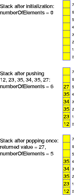
The requirements are more limited than for lists, and therefore we may expect all operations to be performable efficiently. In this context, that means in O(1) time. Stacks are of great importance in many contexts, particularly also in the computer itself: a procedure call results in pushing the current state of the calling routine on the stack, allowing to resume execution here at a later stage after restoring the state.
  public class Stack
  {

    // Invariant: at all times after completion of the routines,
    // numberOfElements always gives the current number of elements.

    private int[] a;
    private int   size;
    private int   numberOfElements;

    public Stack(int s)
    {
      size = s;
      a = new int[size];
      numberOfElements = 0;
    }

    public boolean isEmpty()
    {
      return numberOfElements == 0;
    }

    public boolean isFull()
    {
      return numberOfElements == size;
    }

    public void push(int x)
    {
      if (! isFull())
      {
        a[numberOfElements] = x;
        numberOfElements++;
      }
      else
        System.out.println("Stack full, ignoring!");
    }

    public int pop()
    {
      if (! isEmpty())
      {
        numberOfElements--;
        return a[numberOfElements];
      }
      else
      {
        System.out.println("Attempt to pop from empty stack!");
        return 0;
      }
    }
  }
We work out the details. If we have just started a fresh structure, then we may assume the size of the stack, n, to be half of the size of the array, 2 * n. That is, if we are growing beyond the size of the array, then we have been performing at least n pushes to the stack. That is, creating a new array of double size and copying all the data from the stack into it would cost at most 2 copy operations per performed push operations. If the size of the stack is shrinking, then we are going to create a new array of size n and have to copy the remaining n / 2 elements of the stack into it. It takes at least n / 2 pops before we have to do this. Thus, amortizing these costs, this adds the cost for one copy for every performed pop.
This idea, for x == 2, is implemented in the following program, which can be downloaded here. Notice that by handing over the address of the array to the procedures which adapt its size, we do not really notice the changes which are performed in the subroutines: in main it looks as if we are working with the same array a[] at all times.
[an error occurred while processing this directive]
This program performs pushes and pops in random order, each of the operations being equally likely (a random generator is used to perform coin tosses). Doing this, the stack might grow with each performed operation, but a probabilistic analysis shows that when performing T operations in total, the maximum number of elements on the stack is bounded by Theta(sqrt(T)) with high probability. It may also happen that pops are performed on an empty stack. This program may be understood as an abstraction of some clerk doing work. In principle he is fast enough, but nevertheless, in the course of the years, the pile of work on his desk tends to grow.
The following gives an example output after performing 10^9 operations:
  499985770 pushes
  500014230 pops
     44210 pops on empty stack
   1431770 elements copied
  Maximum size            of stack =  65536
  Average size            of stack =  17001
  Final   size            of stack =  32768
  Maximum number elements on stack =  37610
  Average number elements on stack =   9449
  Final   number elements on stack =  15750
Even though this is only a single example, it is highly representative.
There are two important observations to make:
We work out the idea outlined above. In practice, depending on the distribution of pops and pushes, it may be best to work with green and yellow zones, but the easiest is to start building new structures immediately. As soon as we start working with the new array of size 2 * n, we create a new array: A_s of size n and A_l of size 4 * n. Then, whenever the size of the stack reaches a new maximum value n + x, we copy two more elements from the stack to A_l (the elements with indices 2 * x - 2 and 2 * x - 1). Whenever we reach a new minimum value n - x, we copy one element to A_s (the element with index x - 1). In this way, the copying has just been completed when the stack has 2 * n or n / 2 elements.
Because of the very special (simple) properties of the insertions and deletions to a stack, all this is rather easy. For other data structures, one can often apply the same idea, but not so easily. For a list, to which insertions can be performed anywhere one must be more careful, and updates may also have to be made to the half-ready structure. Actually, for stacks the cost for creating new smaller structures can be saved all together, when we do not throw away the previously used smaller arrays: the contents of these are still valid.
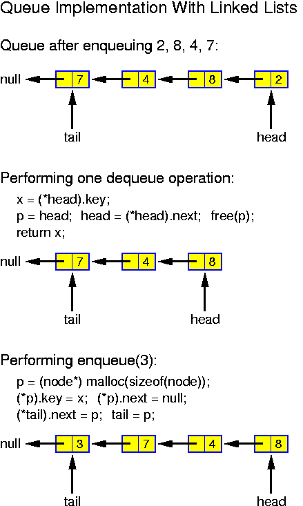
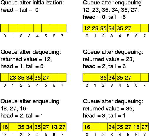
Alternatively, there is a trivial and stupid implementation of queues (which is nevertheless acceptable if the size of the queue is small, say 20): we have an array and maintain as invariant property, that at all times the element to be dequeued, the head of the queue, stands in position 0. This is achieved as follows: when dequeuing, all entries are shifted one position, when enqueuing, the new entry is written at the first free position. Doing this for a queue with n elements, enqueus take O(1) time, while dequeues take O(n) time.
It is not hard to achieve O(1) for both operations. There are variables head and tail. Head indicates the position of the array where the next element can be dequeued. Tail indicates where the next element can be enqueued. Initially we set head = 0 and tail = 0. The following operations then correctly perform the queue operations as long as the array is long enough:
  class Queue
  {

    // Invariant: at all times after completion of the routines,
    // head indicates position to dequeue, tail position to enqueue

    protected int a[];
    protected int size;
    protected int head;
    protected int tail;

    public Queue(int s)
    {
      size = s;
      a = new int[size];
      head = 0;
      tail = 0;
    }

    public boolean isEmpty()
    {
      return tail == head;
    }

    public boolean isFull()
    {
      return tail == size;
    }

    public void enqueue(int x)
    {
      if (!isFull())
      {
        a[tail] = x;
        tail++;
      }
      else
        System.out.println("No space left, ignoring!");
    }

    public int dequeue()
    {
      if (!isEmpty())
      {
        int x = a[head];
        head++;
        return x;
      }
      else
      {
        System.out.println("Attempt to dequeue from empty queue!");
        return 0;
      }
    }
  }
The problem with this approach is that if we are performing many operations, then we will run out off the array, even when the maximum number of elements enqueued at the same time is small. There is a much better construction with arrays, which is hardly more complicated and still guarantees that all operations (as long as the size of the array is sufficiently large to store all elements) can be performed in O(1): head and tail are computed modulo the length n of the array a[]. There are three situations to distinguish:
  class BetterQueue extends Queue
  {

    protected boolean isFull;

    public BetterQueue(int s)
    {
      super(s);
      isFull = false;
    }

    public boolean isEmpty()
    {
      return (head == tail) && !isFull;
    }

    public boolean isFull()
    {
      return isFull;
    }

    public void enqueue(int x)
    {
      if (!isFull())
      {
        a[tail] = x;
        tail++;
        if (tail == size)
          tail = 0;
        isFull = tail == head;
      }
      else
        System.out.println("No space left, ignoring!");
    }

    public int dequeue()
    {
      if (!isEmpty())
      {
        int x = a[head];
        head++;
        if (head == size)
          head = 0;
        isFull = false;
        return x;
      }
      else
      {
        System.out.println("Attempt to dequeue from empty queue!");
        return 0;
      }
    }
  }
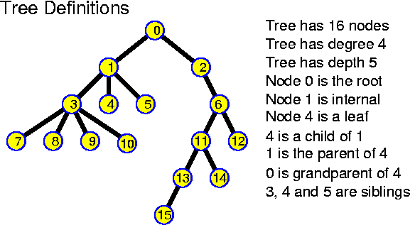
A tree has at least edges pointing away from the root towards the nodes. There may be reasons to have other edges as well: such as edges leading upwards (this adds only one extra pointer to every node, independently of the degree of the tree); or extra links along the leaves. There are many clever ideas in this highly investigated domain.
A tree is realized by creating node objects with as many node objects as required. If the structure of the tree is too irregular to allow a fixed setting, the children must be implemented with a linked list. In our further considerations the trees will mostly be binary, in that case we can just take something like
  class TreeNode
  {
    int      key;
    TreeNode leftChild;
    TreeNode rightChild;
  }
Throughout this chapter, the code examples will be given in a Java-like
style, using TreeNode objects with the above instance variables. For the ternary
trees considered later, we should also have leftChild, middleChild
and rightChild.
Notice that any tree in which all nodes that are not leafs have degree 2 has at least n / 2 leafs. More precisely, such a tree has (n + 1) / 2 leafs. The proof goes by induction. The claim is true for a tree with one leaf. Now consider a tree T with at least one internal node. Let u be one of the deepest lying internal nodes. Because of this choice, both children v and w of u are leafs. Let T' be the tree obtained from T by replacing u and its two children by a single leaf node u'. T' is again a tree satisfying the condition that all non-leafs have degree 2, having n - 2 nodes. So, it has ((n - 2) + 1) / 2 = (n + 1) / 2 - 1 leafs because of the induction hypothesis. Thus, T has (n + 1) / 2 leafs, because it has v and w as leafs instead of u'.
Trees will be used to store information in the nodes, that can be found with help of keys that are used for guiding us on a path down from the root to the information we are looking for. The fact that there are more than n / 2 leaves implies, that if for some reason we prefer to only store information in the leaves, and not in the internal nodes (this may make updates easier), then we can do so at the expense of at most doubling the size of the tree.
So, on a binary search tree (hereafter the word "binary" will be omited, as we will mainly consider binary trees), testing whether a certain key x occurs in the set of stored keys can be performed by calling the following Java method for the root node:
  boolean find(int x)
  {
    if (x == key)
      return true;
    if (x < key)
      if (leftChild == null)
        return false;
      else
        return leftChild.find(x);
    else
      if (rightChild == null)
        return false;
      else
        return rightChild.find(x);
  }
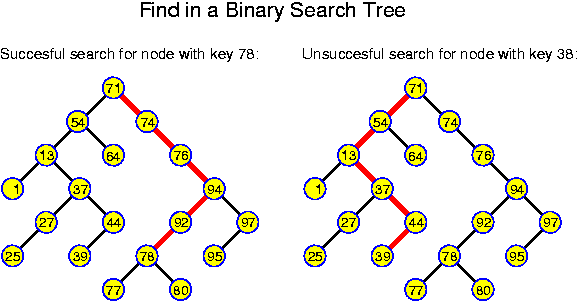
This is interesting. We see that on a search tree, we can perform any find operation in O(depth) time.
In a binary tree each node has at most two children. This immediately gives a simple recurrency relation for the maximum number N(k) of nodes in a binary tree of depth k:
N(0) = 1,Trying a few values gives N(0) = 1, N(1) = 3, N(2) = 7, N(3) = 15. This should suffice to formulate the hypothesis that generally N(k) = 2^{k + 1} - 1. This can easily be checked using induction. More generally, for a-ary trees, we have
N(k) = 1 + 2 * N(k - 1), for all k > 0.
N_a(0) = 1,N_a(0) = 1, N_a(1) = 1 + a, N_a(2) = 1 + a + a^2 and N_a(k) = sum_{i = 0}^k a^k = (a^{k + 1} - 1) / (a - 1). Notice that for all a and k N_a(k) >= a^k, which is easy to remember. So, the number of nodes may be exponential in the depth of the tree.
N_a(k) = 1 + a * N(k - 1), for all k > 0.
A level in a tree is constituted by all nodes at the same distance from the root. Level k of a binary tree T is said to be full if there are 2^k nodes at level k of T. A binary tree is called perfect if all levels are full except possibly the deepest one. Kind of a reversal of the above analysis of N(k) is given by:
Lemma: A perfect binary tree with n nodes has depth equal to round_down(log_2 n).
Proof: A perfect binary tree with 2^k - 1 nodes has depth k - 1: it consists of k full levels. Thus, the perfect binary tree with 2^k nodes must have depth k. At this new level, 2^k nodes can be accommodated. So, any perfect binary tree with n nodes, for 2^k <= n < 2^{k + 1} has depth k. For all these n, we just have that k = round_down(log_2 n).
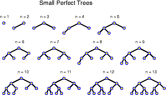
The above tells us that the depth of perfect trees is logarithmic. Of course this does not imply that all trees are shallow: if the root and all internal nodes have degree 1, a tree with n nodes has depth n - 1.
The depth of trees ranges from logarithmic to linear. Therefore, bounding the time of operations in the depth only makes sense if at the same time it is assured that the depth remains somewhat bounded.
As most operations, the depth of all nodes can be computed by a very simple recursive procedure, exploiting the recursive definition of a tree: A tree is empty or it consist of a single node or it consists of two trees linked to a root node. The procedure is called from outside with computeDepth(root, 0). The method returns the maximum depth of any node in the tree, that is, the depth of the tree.
  int computeDepth(int d)
  {
    int m = d;
    if (leftChild != null)
      m = max(m,  leftChild.computeDepth(d + 1));
    if (rightChild != null)
      m = max(m, rightChild.computeDepth(d + 1));
    return m;
  }
  static TreeNode build(int n, TreeNodeSet S)
  {
    if (n == 0)
      return null;
    TreeNode node = S_{n/2};
    node.leftchild  = build(n / 2, subrange(S, 0, n / 2 - 1));
    node.rightchild = build(n - n / 2 - 1, subrange(S, n / 2 + 1, n - 1));
    return node;
  }
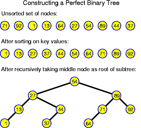
T(1) = cHere we assumed that the splitting of S into the two subsets can be performed in constant time (for example, by only indicating in which range of an array the values lie). The most easy way to proof that the time consumption is linear is by considering the development of the times bottom-up: T(1) = c, T(2) = 3 * c, T(4) = 7 * c. Generally: T(n) = (2 * n - 1) * c. Substitution in the relation shows that this works, formally one should apply induction.
T(n) = c + T(n/2) + T(n/2), for all n > 1
So, we need T_sort + O(n). This is optimal up to constant factors because having the tree we could also read out all elements systematically in sorted order in O(n) time (as is done hereafter), so constructing a search tree must be at least as hard as sorting.
  void inOrderEnumerate()
  {
    if (leftChild != null)
      leftChild.inOrdernumerate();
    print(key);
    if (rightChild != null)
      rightChild.inOrderEnumerate();
    }
  }
The time for this procedure is clearly linear, because processing every
node takes constant time. Alternatively, it may be performed without recursion
with the help of a stack: newly reached nodes are pushed, and when we get stuck
we return to the top element of the stack, that is popped and whose key is
printed on this occasion. This is less elegant but more efficient, because we
save time (no procedure calls) and storage (only the necessary data are pushed
on the stack).
The given inorder enumeration procedure has the nice feature that all keys are listed in increasing order (because of the definition of a search tree). However, we also might want to have different orders. Performing the print operation before the first recursion, gives preorder enumeration; performing it after the second recursion gives postorder enumeration.
On a set of these objects we want to perform the following operations:
Using arrays it is no problem to either perform insert in O(1) and find in O(n), or, when keeping the array sorted at all times, to do the find in O(log n) and the insert in O(n). Trees are the key to greater efficiency. let us first consider how these operations can be implemented, without paying too much attention to the efficiency.
If there are rare updates, then it is a good idea to keep in addition to the tree (or simply the sorted list of elements), a list with "new issues". If an element is added, then it is put in this list. If an element is deleted, then it is marked as deleted in the existing tree. Doing this, a deletion is trivial: the same time as a find. An insertion takes O(1) after testing whether the element is already there. A find takes O(log n + length of additional list). So, this is fine as long as the additional list contains at most O(log n) elements. Because of the extreme simplicity, this may indeed be a good idea in practical cases!
A disadvantage is that every now and then the tree has to be rebuild entirely. However, there is no problem to amortize these costs. The idea is very similar to what we have been doing for queues and stacks implemented array: start rebuilding the tree already before we need the new one.
Even amortizing the cost will not bring us so much: already after O(log n) additions, we may need a new tree. This new construction costs us O(n) (most keys are already sorted), so n / log n per performed insertion. Thus, only if we perform many more finds and deletes than insertions (the factor is n / log^2 n), this works well.
Actually, this whole idea has been applied for centuries in the context of printed media. Think of an encyclopedia: the original work appears, soon followed by a list of errata. Then, every year, updates are added. The speed at which information can be found goes down with every update. Finally a completely new issue appears and the process begins again. One of the biggest advantages of the use of electronic storage devices is that information can be changed or deleted without leaving traces.
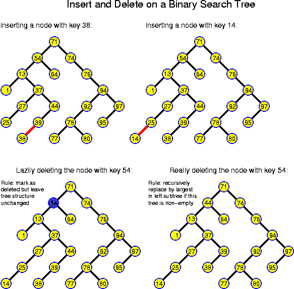
Inserting a node to a tree of which we have access to the root can be performed by calling the following Java method form outside with root.insert(node):
  void insert(TreeNode node)
  {
    if (node.key  == key)
      printf("Key already exists\n");
    else
      if (node.key < key)
        if (leftChild == null)
          leftChild = node;
        else
          leftChild.insert(node);
      else
        if (rightChild == null)
          rightChild = node;
        else
          rightChild.insert(node);
  }
The simplest general solution is to perform lazy deletions: a node to delete is marked by setting an additional boolean instance variable of TreeNode to false. Otherwise the node is left unchanged. This idea guarantees to not impair the search-tree property because the key of a deleted node is still available for guiding the search through the tree. So, the only change to the procedure find is to test whether a node with key == x is deleted or not before returning true. When inserting a node with a key x, while a deleted node with key x is still present in the tree, then the deleted node should be replaced by the new one. Any newly inserted node gets its mark set to true.
This is a very good solution if we have a finite set of elements which are repeatedly inserted and deleted. However, in that case we can better use a sorted array, which is even simpler. More generally, this idea has the problem that over time the structure may become more and more polluted. The obvious solution is to rebuild the tree without the deleted nodes as soon as their number exceeds 50% (or some other constant fraction) of the total number of nodes. This implies a certain waste of memory space, but typically it has very little impact on the time for searching: if we can guarantee that the depth of a tree with n nodes is bounded by c * log n, for some constant c, then the time to search in a tree with n real nodes polluted with at most n deleted nodes is c * (log n + 1) instead of c * log n for a clean tree.
The rebuilding is not too expensive: performing an infix tree traversal, all non-deleted nodes can be extracted from the tree in sorted order in linear time. Building a new perfect tree out of these takes linear time as well. If the resulting structure has n nodes, then at least n / 2 delete operations can be performed before the next rebuilding. Thus, the rebuilding has an amortized cost of O(1) per operation.
As noticed above, a node u can be directly removed from the tree only when u is a leaf. In all other cases this would cut the tree. If u has degree 1, then its single child may be attached directly to its parent. If u has degree 2, attaching both children to its parent would increase the degree of the parent, which is not allowed in the case of binary trees we are considering here.
The general solution is to find a replacement v for u. The key of v should be such that all nodes in the left subtree have smaller values and all nodes in the right subtree larger values. The largest key value m in the left subtree has the desired property: by definition m is larger than all other keys in the left subtree, and because we may assume (induction) that so far the tree had the search-tree property, m is smaller than all keys in the right subtree. Also the smallest key value from the right subtree has the desired property. The problem is that the node v with key m is not necessarily a leaf itself. However, v certainly lies deeper than u, and thus this may be overcome by performing the replacement recursively, until we have reached a leaf.
In Java-like code the idea can be realized as follows:
  TreeNode findFather(int x)
  {
    if (x < key)
    {
      if (leftChild == null || leftChild.key == x)
        return this;
      return leftChild.findFather(x);
    }
    else
    {
      if (rightChild == null || rightChild.key == x)
        return this;
      return rightChild.findFather(x);
    }
  }

  void delete(key x)
  {
    TreeNode w = findFather(x);
    TreeNode u; // the node to delete
    if (x < w.key)
      u = w.leftChild;
    else
      u = w.rightChild;
    if (u == null)
      printf("No node with key " + x + " in the tree");
    else // there is a node with key x to delete
    {
      if (u.leftChild == null && u.rightChild == null)
        if (x < w.key)
          w.leftChild = null;
        else
          w.rightChild = null;
      else // u is not a leaf
      {
        TreeNode v;
        if (u.leftChild != null)
          v = (u.leftChild).findFather(MAXINT);
        else
          v = (u.rightChild).findFather(- MAXINT);
        u.key = v.key;
        u.delete(v.key);
      }
    }
  }
The method findFather returns the father of the node with the value we are
looking for, or, if this value not occurs, the node where the link leading to a
node with key x is missing. The same method is also used for finding the node
with largest /smallest key in a subtree. In delete we have been careful to even
handle the case that v is a child of u correctly.
The above shows that the time consumption for all three operations is bounded by O(depth of tree). As long as the tree is as it should be: balanced in the sense that for n nodes the maximum depth is bounded by O(log n), we are happy. However, very natural operations may lead to trees that are degenerated: having depth omega(log n). This already happens when the elements are inserted in sorted order: all elements are inserted as right childs, leading to a tree with the structure of a linear list.
If it can somehow be guaranteed that the tree remains balanced in the dynamic context of insertions and deletions, then all operations can be performed in O(log n) time.
In Java the sentinel idea might be implemented as follows:
  class TreeNode
  {
    int key;
    TreeNode  leftChild;
    TreeNode rightChild;

    TreeNode(int key)
    {
      this.key   = key;
      leftChild  = null;
      rightChild = null;
    }

    // All other previously given methods
  }

  class Tree
  {
    TreeNode root;

    Tree()
    {
      root = new TreeNode(MAXINT);
    }

    static Tree build(int n, TreeNodeSet S)
    {
      Tree tree = new Tree();
      root.left = TreeNode.build(n, S);
    }

    int computeDepth()
    {
      root.findDepth(-1);
    }

    int inorderEnumerate()
    {
      if (root.leftChild == null)
        printf("Tree is empty\n");
      else
        (root.leftChild).inOrderEnumerate();
    }

    boolean find(int x)
    {
      return root.find(x);
    }

    void insert(TreeNode node)
    {
      root.insert(node);
    }

    void delete(int x)
    {
      root.delete(x);
    }
  }
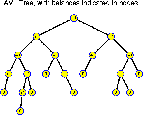
The balance of a node is the difference between the depth of the left and right subtree. The balance can be computed easily by a modification of the method computeDepth(). A node is said to have the AVL property, if its balance is -1, 0 or 1. A tree is said to be an AVL tree if all its nodes have the AVL property. This definition leaves considerable flexibility. One of the positive aspects is that the AVL property is local, this implies that an insertion or deletion only has impact for the nodes along the search path. Any perfect tree is an AVL tree, but an AVL tree does not need to look like a perfect tree at all: the leafs may lie at many different levels. A priori it is neither clear that the depth of such trees is bounded to O(log n) nor that we can perform inserts and deletes on AVL trees without needing reconstructions that cost more than O(log n) time.
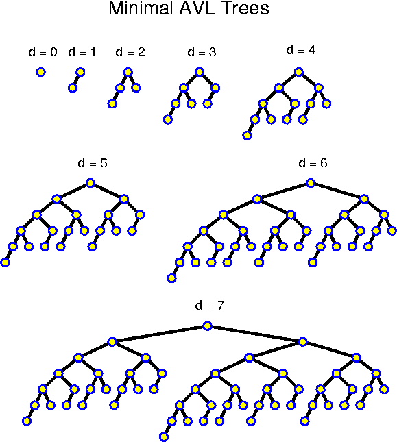
N(-1) = 0,Thus, the N(d) are very similar to the Fibonacci numbers, and even slightly larger. How do these numbers develop exactly? We have N(0) = 1, N(1) = 2, N(2) = 4, N(3) = 7, N(4) = 12, N(5) = 20, N(6) = 33, N(7) = 54, N(8) = 88, N(9) = 143, N(10) = 231, ... . We see that they grow fast! Actually, looking at them we get the strong feeling that they grow exponentially, even though they do not double every step.
N(0) = 1,
N(d) = N(d - 1) + N(d - 2) + 1, for all d > 1.
How can one prove such a fact? In (almost) all such cases, one should use induction. For induction we need an induction hypothesis. The problem here is that we do not know exactly what we want to prove. If we just want to prove that the development is exponential, we can use an underestimate. It is easy to check that all N(d) are positive. From this it follows that N(d) > N(d - 1) for all d > 1. Thus, N(d) > 2 * N(d - 2). So, as an hypothesis we could use N(d) >= sqrt(2)^d. We must check the basis of the induction. This is ok, because sqrt(2)^0 = 1 <= N(0), and sqrt(2)^1 = sqrt(2) <= N(1). After that we must only check that indeed N(d + 2) > 2 * N(d) >= 2 * sqrt(2)^d = sqrt(2)^{d + 2}.
In principle this is good enough. If, however, we want a more accurate estimate, then we can do the following which is a special case of an approach that works in general for estimating the exponential development of a recurrency relation. We assume that the development is as a^d, for the time being we forget about constant factors and additional terms. How big is a? Because the exponential behavior dominates all other things, we should basically have a^d = a^{d - 1} + a^{d - 2}. Dividing left and right side by a^{d - 2} gives a quadratic equation: a^2 - a - 1 = 0. Solving with the ABC-rule gives a = (1 + sqrt(5)) / 2 +-= 1.618, the famous golden ratio. For the ancient Greeks (particularly the Pythagoreans), and throughout the history of art, this number meant utter harmony. For this one can repeat the above induction proof. We are lucky that we have "+ 1" and not "- 1". Otherwise the development would still have been of the same order, but the proof would have been harder. So, we know now that the depth of an AVL tree with a given number of nodes N is at most log_a N = log_2 N / log_2 a = 1.440 * log_2 N. In most cases it will be less, but the main point is that this is logarithmic.
The problem is that we must somehow guarantee that the tree is again an AVL-tree afterwards. Otherwise we could soon not guarantee anymore that the depth of the tree is logarithmic, and all our time bounds are based on that assumption.
Another observation is that a single insertion can change the depth of any subtree by at most one. So, if after the insertion there are nodes in unbalance, then this is because one of their subtrees has depth exactly 2 larger than the other subtree.
Let w be the deepest node with unbalance. Without loss of generality we may assume that the left subtree of w, rooted at w_l is too deep in comparison to the right subtree rooted at w_r. More precisely, we assume that the balance of w is +2. The subtrees of w_l are denoted by w_ll and w_lr. Possibly these subtrees are empty, but at the level of this theoretical discussion it does not matter. It helps to consider the performed operations in an abstract way.
A crucial observation is that the tree was balanced before the insertion. Because now the depth of the subtree of w_l is two larger than that of w_r, it must have been exactly one larger before. The insertion must have changed the depth of w_l, and consequently of either w_ll or w_lr, otherwise the balance would still be ok. In order to increase the depth of a tree, one must perform the insertion in the subtree whose depth is larger or equal than the other. If this depth would have been larger already before the insertion, then it would now be larger by two. But, if the depth of either w_ll or w_lr exceeds the other by two, then w_l is unbalanced after the insertion, in contradiction with our assumption that w is the deepest unbalanced node. So, now we know incredibly precisely how the tree looked before and after the insertion:
The subtrees rooted at w_ll, w_lr and w_r all had the same depth. As a result of the insertion, the depth of w_ll or w_lr has increased by one.
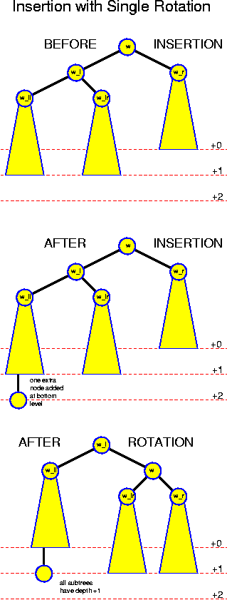
The first case is the simplest. In that case, we make w_l to the new root of this subtree, hook w to it as right child and w_ll as left child. w gets as right child w_r and as left child w_lr. The ordering is preserved by these operations, and after this, the balance has become perfect, because the tree of w_ll has moved one level up, and the tree of w_r has moved one level down. This operations is called single rotation.
This operation works because the subtree rooted at w_ll, whose increased depth was the cause of all trouble, is on the outside. So, it remains attached to w_l, which is lifted, so it is lifted along. Thus, this effectively reduces the depth of the left subtree. The depth of our right subtree, which was two smaller, so it now becomes equal. The subtree rooted at w_lr is thrown over to w_r. Because w_r now has the same level as w_l before, its depth remains unchanged. We conclude that afterwards all depths are the same.
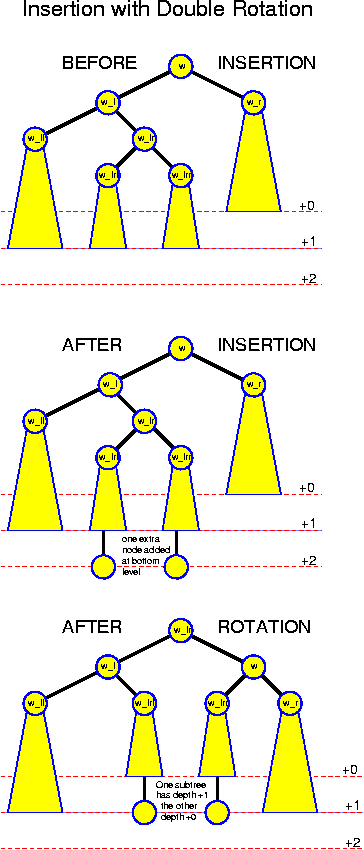
So, we must apply a more elaborate technique called double rotation. the idea is now to make w_lr the root of a newly constructed subtree with w_l as its leftchild and w as its rightchild (among other things you should notice that indeed the key of w_lr is larger than that of w_l and smaller than that of w). w_l gets new children w_ll and w_lrl; w gets new children w_lrr and w_r.
Remember that in this case w_lr is turned into the new root. Once you have decided to do this, the requirement that the tree remains ordered does not leave you any other option but rearranging as described.
The subtree that was deepest, the one that was rooted at w_lrl or w_lrr is indeed raised one level by this operation (because these nodes now come at distance two from the root, whereas before this was three). The subtree of w_ll remains at the same level, and the subtree of w_rr is going down one level, but this is fine. So, afterwards, we have three of the four subtrees at the same level, and one of them one less.
Actually, there is no need to implement two different routines, because single and double rotations are not so different as they appear. In both cases, starting at w, the search path is followed down for two steps. This gives a set of in total three nodes: w, w_x and w_xy, Here x and y stand for 'l' or 'r'. In each of these four cases, these three nodes are used to construct the top of a tree of depth 1. The node with smallest key appears as left child, the node with largest key appears as right child. The four involved subtrees (one from w, one from w_x and two from w_xy) are attached to the two leafs of this small tree in the same order as before. Ignoring the difference between single and double rotations saves a case distinction and a subroutine at the expense of slightly increased costs for the single-rotation case.
If the balance remains within the acceptable bounds, then we are ready. Otherwise, we look for the deepest node w whose balance is no longer ok. From the fact that w was ok before the deletion, we conclude that one of the subtrees of w, say the right one, has depth exactly two smaller than the other. Denote by w_l and w_r the left and right child of w, and by w_ll, w_lr, w_rl and w_rr the grandchildren. The depth of w_r must have been reduced. Because it was balanced before, the deeper of its subtrees must have had depth exactly one larger than the other, and thus now the trees rooted at w_rl and w_rr have the same depth. For the depths of the trees rooted at w_ll and w_lr there are three possibilities: (+2, +1), (+1, +2) and (+2, +2). Here a number +x denotes how much deeper this subtree is than the trees rooted at w_rl and w_rr. There must be a +2 because w is unbalanced now and there cannot be anything else because w was balanced before.
The treatment of these cases is completely analogous to what we have done before. The simplest case is again (+2, +1). Then it is sufficient to perform a single rotation: w_l becomes the new root. w becomes its right child. w gets w_lr as new left child.
The case (+1, +2) can be treated with a simple double rotation: w_lr becomes the new root, with w as right child and w_l as left child. w has w_r as right child and w_lrr as left child. w_l has w_lrl as right child and w_ll as left child.
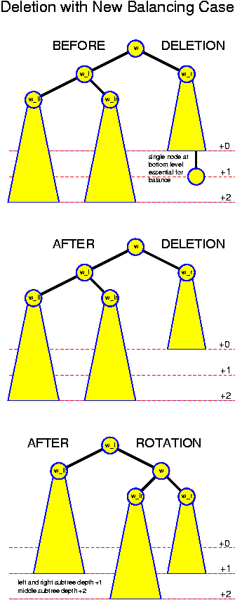
The only really new case is (+2, +2). Fortunately, performing a single rotation, helps in this case: single rotation makes the subtree rooted at w_r one deeper, the subtree rooted at w_ll becomes one undeeper, and the subtree rooted at w_lr remains at the same level. This operation is illustrated in the following picture:
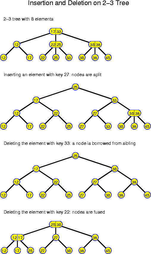
In this case, the internal nodes typically do not hold information, but one or two keys that guide the searching process. If there is one key k, then k could be the largest value of the left subtree. If there are two values k_1 and k_2, then k_1 is the largest value of the left subtree and k_2 the largest value of the middle subtree.
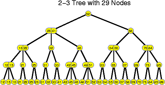
  if      (x <= k_1)
    goleft();
  else if (x <= k_2)
    gomiddle();
  else //  x >  k_2
    goright();
In this way we continue until we reach a leaf. There we test whether the
key is equal or not and perform a suitable operation in reaction.
The construction and these more elaborate comparison imply a certain overhead, but all the rest becomes much simpler because of this. If you would implement a search tree ADT based on 2-3 trees, then it is a good idea to have different classes for internal nodes and leafs, as they allow very different operations and have different fields as well.
It is essential that 3 + 1 = 2 + 2. This implies that, once the maximum degree of a node is exceeded, it can be split in two nodes with degree within the legal range. This implies that we could make a 3-5 tree in the same way, because 5 + 1 = 3 + 3, but that a 3-4 tree would be clumsy, because 4 + 1 = 5 < 3 + 3. These generalizations are called a-b trees. The degrees of the nodes lie between a and b and we must have b + 1 >= 2 * a. 2-3 trees have the problem that after splitting a node (as the result of an insertion) the new nodes have degree 2, which is the minimum. Therefore, it may happen that a subsequent deletion immediately leads to a fusion again. These structural changes may go all the way up to the root every time. Even though all these takes only logarithmic time, it still will mean a considerable increase of the cost. If we would use 2-5 trees instead, then after a splitting operation we obtain nodes of degree 3, which are not critical, and which cannot be split immediately afterwards. For 2-5 trees one can even show that the amortized number of restructuring operations is constant.
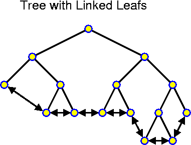
This can be realized in several ways, but one very simple way is based on search trees. First we assume that the information is only stored in the leafs of the tree and that the leafs are connected in a doubly linked way to each other (if for the leafs we use the same objects as for the internal nodes, then we have some spare links, which can be used for this!). In this case we search for x_low and then walk along the leafs until hitting x_hgh or a larger value. This whole procedure takes O(depth of tree + number of nodes in the range). This is clearly optimal, because any search takes at least O(depth of tree) time and handling all elements takes at least O(number of nodes in the range).
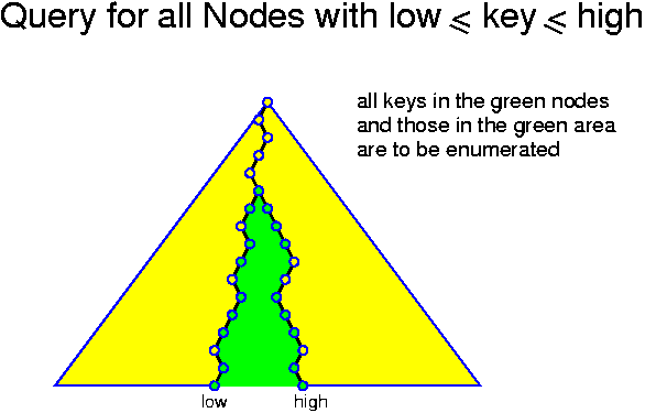
Range queries can also be performed on a conventional binary tree with the information stored in all nodes. The idea is to walk down the tree until x_low and x_hgh do no longer follow the same path. Then, whenever the search for x_low moves left in a node u, u and all keys in its right subtree should be enumerated. Analogously, whenever the search for x_hgh moves right in a node v, v and all keys in its left subtree should be enumerated.
One of the subsequent chapters is entirely devoted to priority queues. Here we consider a basic realization with search trees in which the priorities are used as keys. On this structure insert is trivial: use the insert operation of the search tree.
An operation that can be implemented very easily on search trees is "find the node with smallest key": just walk left all the time until hitting a node without left child. Thus, the following can be used to implement a deletemin:
  x = searchTree.giveSmallest();
  searchTree.delete(x);
  return x;
Decreasekey is also simple: go to the specified node, delete it from the search tree and reinsert it with modified priority. The only problem is that typically the node of which the priority should be modified is typically not specified by its priority but by another tag. For example, if we are managing the waiting list of a hospital, a typical instruction will not be decreaseKey(89, 74), but rather decreaseKey("Baker", 74), indicating that the priority of "Baker" should be set to 74. The solution is to use a second search tree in which the names are used as key.
The simplest realization of this idea is to have two trees in which all nodes have two keys. One tree is ordered according to the priorities, the other according to the names. Inserts are performed in each tree. For a deletemin, one searches the node with minimum priority in the tree which is ordered according to the priorities. There one finds the corresponding name which can subsequently be searched for in the other tree. When performing a decreasekey, one first searches for the name in the tree which is ordered according to the names, there one finds the corresponding priority which can subsequently be searched for in the other tree. In this way the information in both trees remains the same after completion of each operation.
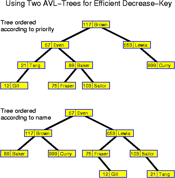
The same idea can be realized more efficiently if there are links from one tree to the other in both directions. In that case decreaseKey("Baker", 74) is performed by searching for "Baker" in the name tree and then following the link to the node with its priority in the other tree. When performing deletemin one searches in the tree with priorities for the smallest key. From there one follows the link to the other tree. The structure is more complex, but the additional links reduce the time for finding the element in the second tree.
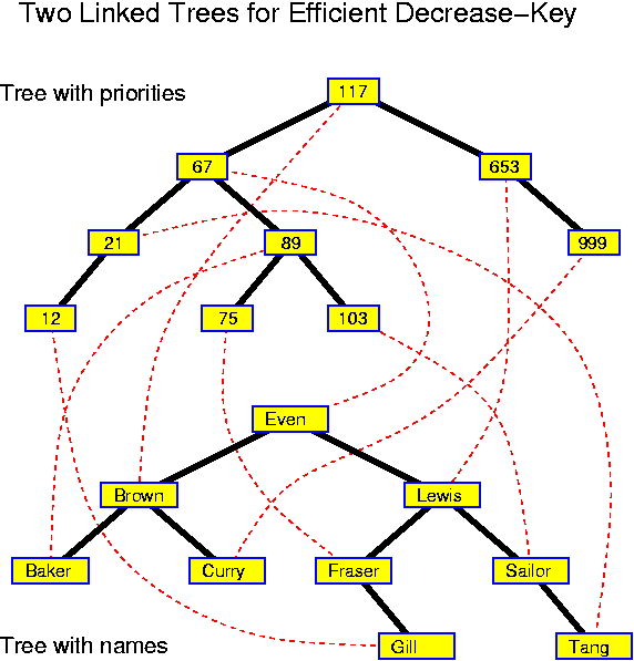
Each of these realizations assures that, as long as we use one of the balanced search trees, all three priority-queue operations can be performed in O(log n) time. This is not the best achievable, but quite acceptable. As we will see, either insert or deletemin must take Omega(log n) time.
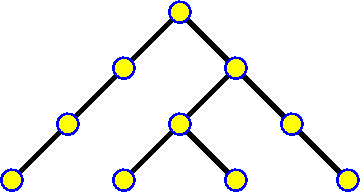
The canonical way of implementing this ADT is, as the name suggests, by using a search tree, but this is not the only possible way. If we really only want to implement the above three operations, then there are alternative ways, that are
  void insert(int k) {
    a[k] = true; }

  void delete(int k) {
    a[k] = false; }

  boolean find(int k) {
    return a[k]; }
Of course, in most real-life applications some additional information will
be stored along with the entry in a[], but this holds for any of the discussed
data structures: here we focus on how to perform the basic operations. This
special case is not called hashing, but direct addressing. The name is
inspired by the fact that the key values are directly, without any modification,
used for determining where data are stored. Its efficiency essentially depends
on the availability of RAM.
Direct addressing is based on the same underlying idea as bucket sort. Like bucket sort, direct addressing is applicable only for moderate M. There is a difference with bucket sort though: bucket sort even requires O(M) time, whereas direct addressing, applying virtual initialization, only requires sufficient memory.
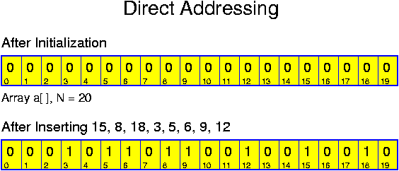
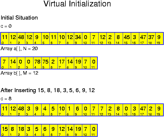
More generally, we have at most N numbers from 0 to M - 1. Then we have one integer array a[] of size M and one integer array b[] of size N plus one counter c, giving the number of inserted elements, initially with value 0. To insert an element k, we perform
  void insert(int k) {
    a[k] = c;
    b[c] = k;
    c++; }
To check whether x is there we perform
  boolean find(int k) {
    if (a[k] >= c)
      return false;
    else
      return (b[a[k]] == k); }
Deletions are simple to perform:
  void delete(int k) {
    a[k] = c; }
One might also use any other value which is guaranteed not to be equal to
the original value of a[k]. A disadvantage is that the entry in b[] is not
removed. So, if insertions and deletions are alternated then c will increase to
a value larger than M.
This is unnecessary, the unused space can be made available again by a slightly more complicated delete procedure. In this procedure, the last inserted element is deleted and reinserted at the position of k:
  void delete(int k) {
    a[b[c - 1]] = a[k];
    b[a[k]] = b[c - 1];
    c--; }
If we compare with the simple approach in which the values are first initialized, then we see that now all operations are more expensive by a small constant factor. A larger disadvantage is the additional memory usage: Before we had one array of N bits. Now we have two arrays with N and M integers, respectively. Even when we may assume that M is much smaller than N (otherwise the whole idea of virtual initialization does not make sense), this is considerably more. Therefore, virtual initialization appears to be a nice idea with limited practical interest.
Suppose for a second that f maps the keys injectively to {0, ..., N - 1}, that is, for any two keys k_1 and k_2, f(k_1) != f(k_2). Then we have a great search structure: the three operations can be performed in constant time almost just as with direct addressing. The main difference is that instead of accessing position k, we must access position f(k):
  void insert(int k) {
    a[f(k)] = k; }

  void delete(int k) {
    a[f(k)] = -1; }

  boolean find(int k) {
    return a[f(k)] == k; }
There is one more difference with direct addressing: because many values
may be mapped to the same position, it does not suffice to set a boolean. It is
essential to mark a position by the key itself, so that when performing a find
it can be tested whether it was really k that was mapped here or some other
value k' with f(k') == f(k). Thus, a[] must be an integer array. Just as with
direct addressing, the efficiency of hashing depends on the availability of RAM:
once we know the index we can go to the desired position in the array without
noticeable delay.
Because the keys are not known beforehand, we cannot hope to choose the hash function f in an optimal way, avoiding all collisions. Such a function might also be expensive to compute. The best we can reasonably hope for is that f is as good as randomly scattering the elements over the array. We cite some basic facts from probability theory:
In Java, with objects of a type ListNode with fields key and next, the chaining idea can be implemented as follows:
  void insert(int k) {
    a[f(k)] = new ListNode(k, a[f(k)]); }

  void delete(int k) {
    int i = f(k);
    if (a[i] != null) { // not an empty list
      if (a[i].key == k)
        a[i] = a[i].next;
      else {
        ListNode prev = a[i];
        ListNode node = a[i].next;
        while (node != null && node.key != k) {
          prev = node;
          node = node.next; }
        if (node != null)
          prev.next = node.next; } } }

  boolean find(int k) {
    ListNode node = a[f(k)];
    while (node != null && node.key != k)
      node = node.next;
    return node != null; }
This implementation is complicated by the fact that when deleting we must
take care of the special case of empty lists. Working with sentinel elements
costs extra memory, but makes the operations somewhat easier. Click here
to see the above piece of code integrated in a working Java program.
The most expensive operation is an unsuccessful find or an attempt to delete a non-existing element: in these cases the whole list must be traversed. For a successful find we only have to traverse half the list on average. In the typical case that the number of finds exceeds the number of inserts, it may be clever to invest slightly more when inserting elements in order to make the finds cheaper: if the lists are kept sorted, then a find can be terminated as soon as we reach a node with key k' > k.
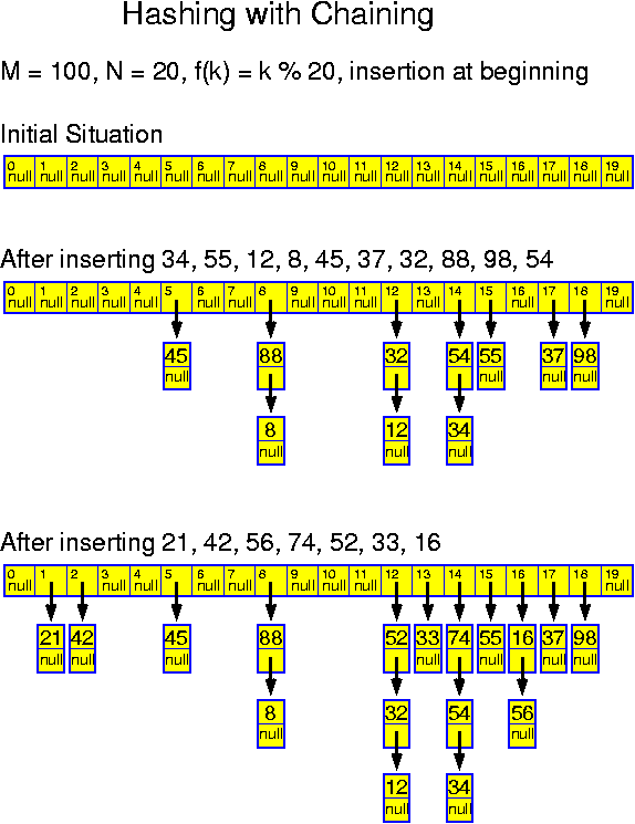
We give an example. Suppose we would like to build a data base for the about one million inhabitants of northern Sweden. More precisely, for the inhabitants of the five provinces (län) which constitute Norrland: Gävleborgslän, Västernorrland, Jämtland, Västerbotten and Norrbotten. As key we use the personal number and the array has length N = 1,000,000. The first six positions of the Swedish personal number consists of the date of birth (in the format yymmdd). Position 7 and 8 indicated until recently the län in which the person was born and only the two last digits are slightly arbitrary (though the gender is encoded in these). If we now simply use f(k) = k mod N, then we will get a very poor distribution: most people living in Norrland are born in this area, so most people are sharing the same 5 possibilities for digit 7 and 8. Furthermore, there are only 31 days, so digits 5 and 6 have only 31 values. Thus, the big majority of the one million people is going to be mapped to at most 15.000 positions, at least 60 for each slot. In this case it is quite obvious and we know an easy way out. Out of the personal number, we should first construct a condensed number, taking into account that there are only 365 days, and 6 län (GL, VN, JL, VB, NB, aliens), and not all final two digits. This would give us a condensed number of size 100 * 365 * 6 * ??. This number we could take modulo N to find the position. In general this is much harder: if we would like to apply hashing to a dictionary of words, then it is clear that not all letters are equally frequent (14% of the Swedish dictionary starts with "s"), but it is hard to do something with such observations.
Not knowing the structure of the numbers we can never guarantee that the chosen hash function is good, however, this can be made independent of the input. The idea is to choose the hash function uniformly from a large class of good hash functions. Even though for any particular hash function there are sets of keys which are mapped to few different positions, it can be achieved in this way that the a priori probability that any two keys k_1 and k_2 are mapped to the same position is exactly 1 / N, that is, just as if they are randomly scattered over the array. This idea is called universal hashing.
Problems may occur but mostly we will be lucky. In that case the elements are distributed more or less evenly. Consider the case that the number of distributed elements n equals the size of the array N. Some longer lists will occur, but most elements are close to the root of their list. If the element to search for is selected uniformly from among the n elements, then it can easily be shown that the expected time for a find operation is constant. Then this also holds for deletes and the time for inserts is constant independently of the length of the lists. The statement may be strengthened further: every individual find may take O(log n) time, but with high probability the time for a sequence of log n finds for independently selected keys is bounded by O(log n) as well. Thus, amortizing over O(log n) operations, the time per operation is O(1) with high probability.
An alternative is to store elements in the array itself. For a while this works fine, but what do we do when an element gets mapped to a position that is already taken?
How could we do a find in this case? We go to f(k). If it is empty we are done. If we find k as well. But, if f(k) is occupied by another element, then we do not know anything. We must continue until we either find k or an empty element. When performing deletions we have to be careful: simply removing an element k does not work. It may namely be the case that other elements which lie after k become unfindable when we would remove k. Therefore, we should perform lazy deletion by somehow marking k as deleted. When performing a find these deleted positions are handled as filled positions, when performing subsequent inserts, they are handled as empty positions, reusing the memory. This technique works fine because the memory space is available anyway.
If all key values are positive, the above ideas may be implemented as follows:
  // -1 means empty
  // -2 means deleted

  void initialize() {
    for (i = 0; i < N; i++)
     a[i] = -1; }

  void insert(int k) {
    for (i = f(k); a[i] >= 0; i = (i + 1) % N);
    a[i] = k; }

  void delete(int k) {
    for (i = f(k); a[i] != k && a[i] != -1; i = (i + 1) % N);
    if (a[i] == k)
      a[i] = -2; }

  boolean find(int k) {
    for (i = f(k); a[i] != k && a[i] != -1; i = (i + 1) % N);
    return a[i] == k; }
Click here
to see slightly modified code integrated in a working Java program. This program
is conceived so that it can be modified very easily to work for the better
conflict-resolution strategies presented in the following.
Not all simple ideas are good ideas. Linear probing has lousy performance once the array becomes slightly fuller. In this relation we need the term load factor, which is the ratio n / N. Mostly expressed in %. So, if we say that the hash table has a load factor of 80%, we mean that we are storing n = 0.8 * N keys in an array of length N. The problem with linear probing is that once we have a small sequence of consecutive positions that are full, that then it is quite likely that the next insertion hits this chain. So, chains tend to grow very fast. This problem is called primary clustering. More precisely, it means that all elements that get mapped to any of the positions of a cluster will make the cluster larger.
Without going into detail we look at some numbers. Suppose we have an array of length 100. Suppose we have inserted 20 elements. Suppose all elements are still isolated (this is quite unlikely). For isolated elements, the probability that they are hit and that the length of their chain becomes 2 is 0.01. If this happens (20% probability, so within a few insertions it will indeed happen), then hereafter, the probability that the chain gets hit is no longer 0.01, but 0.02. When it is hit, the probability becomes larger again. In addition, if the array gets fuller, one large chain may swallow the following chain, further increasing the rate at which chains are growing. A simulation, generating uniformly distributed random numbers in the range 0, ..., N - 1, shows that the load factor should be at most 60 or 70%. Otherwise the performance breaks down. This means that we must always waste at least 30 to 40% of the memory.
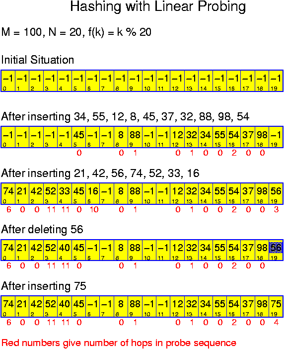
  void insert(int k) {
    for (t = 0; a[p(k, t)] is occupied; t++);
    a[p(k, t)] = k; }
Here p(k, t) gives the probe sequence of k. For linear probing, p(k, t) =
(f(k) + t) mod N. The next simplest idea is to try p(k, t) = (f(k) + t^2) mod N.
This, or similar variants, is called quadratic probing.
Linear probing had the problem of primary clustering, the problem that any key mapped to any position in a chain follows the same trajectory through the array. This leads to a self reinforcing clustering in which the clusters tend to grow very fast. With quadratic probing, we have a less serious form of clustering: all keys that get mapped to the same position f(k) follow the same trajectory. This is called secondary clustering. Primary clustering is worse because it arises even if the hash function distributes the keys over the array completely uniformly. Secondary clustering is a problem only when there are many key values k with the same f(k).
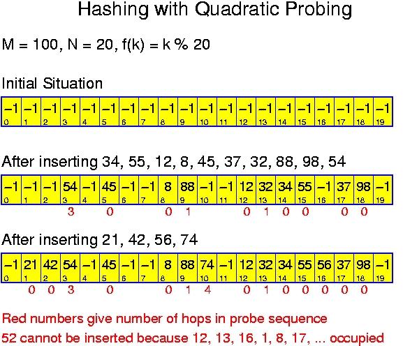
The first point implies that we should not take a simple modulo function. The second point implies that for all k, f_2(k) should be relatively prime to the size N of the hash table. This is most easily assured if N itself is a prime number, then f_2 can assume any value different from multiples of N. If f_1(k) = k mod N, then f_2 can be based on k / N. For example, f_2(k) = 1 + (k / N) mod (N - 1).
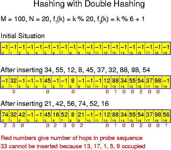
Of course we can continue inserting until the array is entirely full, but this is not clever: the last insertions will cost linear time. The simplest criterion for rebuilding is the load factor. For example, one can rebuild as soon as the load factor exceeds 80%. This is quite static though and does not tak into account that sometimes we are running into bad hashing behavior because of an unlucky choice of the hash function. Therefore, it is better to rebuild as soon as performance becomes too poor. For example, one can rebuild as soon as the latest 1000 insertions took more than c * 1000 steps.
If it is important to keep the maximum time per operation bounded, then the rebuilding can be started somewhat earlier and run in the background until the new structure is ready. In this way the amortized cost of the rebuilding can be reduced to O(1).
The above leaves much freedom in how to perform the unions and how to choose the names. A possibility is to apply a rule like "add first to second", meaning that an operation union(x, y) is performed by adding all elements of the subset in which x lies to the subset in which y lies. The new name for this set then becomes the name of the subset in which y lies.
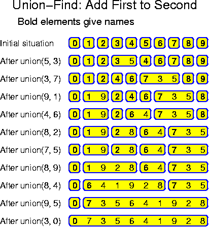
The subset ADT may sound unimportant, but it shows up everywhere. Subsets are the canonical example of the mathematical concept of equivalence relations. An equivalence relation is a binary operator "~" on elements of a set with the property that
The subset ADT allows to maintain equivalence relations dynamically: relations may be added by applying the union operation. The only limitation is that there is no de-union: once unified, the sets cannot be split anymore. This latter feature would be much more expensive to implement, in particular it would require that all previous operations are recorded.
There are several implementations, ranging from extremely simple giving modest performance (one operation O(1), the other O(n)), to slightly less simple giving excellent performance (almost constant time for both operations).
A union is more complicated: if all the elements of a subset S have to be renamed, then, in the simplest implementation, we have to scan the whole array to find those which belong to S. This takes O(n) time. Thus, for all n - 1 unions (after n - 1 non-trivial all elements have been unified into one set ), we need O(n^2) time.
  void initialize() {
    for (int i = 0; i < n; i++)
      a[i] = i; }

  int find(int k) {
    return a[k]; }

  void union(int k1, int k2) {
    k1 = find(k1);
    k2 = find(k2);
    if (k1 != k2) // rename all elements in subset of k1
      for (int i = 0; i < n; i++)
        if (a[i] == k1)
          a[i] = k2; }
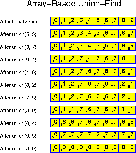
If we are slightly more clever, we might maintain the elements that belong to a set in a linked list. In that case, we do not have to scan through all the elements when performing a union operation. A union is now performed by traversing one of the lists, accessing a[i] for each listed element i and updating it with the index of the other set. Then this list is hooked to the other list.
We consider an implementation of this. The lists are also implemented in an integer array b[]. In general the value b[i] gives the successor of i in its list. It is convenient to maintain a set of circular lists. The initial situation for this can be established by setting b[i] = i, for all 0 <= i < n. These ideas are worked out in the following piece of code:
  void initialize() {
    for (int i = 0; i < n; i++)
      a[i] = b[i] = i; }

  int find(int k) {
    return a[k]; }

  void union(int k1, int k2) {
    int i, j;
    k1 = find(k1);
    k2 = find(k2);
    if (k1 != k2) { // rename all elements in subset of k1
      i = k1;
      do {
        a[i] = k2;
        j = i;
        i = b[i]; }
      while (i != k1);
      // glue list of k1 into the list of k2
      b[j] = b[k2];
      b[k2] = k1; } }
At a first glance this appears to be a very good idea: the implementation is simple and does not cause too much overhead. The work of a union is now proportional to the number of renamings that is, it is proportional to the size of the subset of k1 and no longer Theta(n).
However, consider the following sequence of unions
  for (int i = 1; i < n; i++)
    union(i - 1; i)
If always the first set is joined to the second, then in total we have to
rename sum_{i = 0}^{n - 1} i = (n - 1) * n / 2 = Omega(n^2) elements. This is
half as much as with the trivial implementation, and in view of the extra work
for each renaming, it is actually no improvement at all.
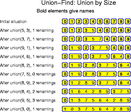
How do we prove such a thing? In this case the idea is to consider the maximum number of times that any node may be given a new name. We show that this happens at most log n times. Then it follows that in total there are at most n * log n renamings.
Lemma: A node that has been renamed k times belongs to a set of size at least 2^k.
Proof: To be formal, we use induction. We must check a base case and a step. The base case is easy: a node that has been renamed 0 times belongs to a set of size at least 1 right from the start. Now suppose the lemma holds for k. Consider a node e that has been renamed k + 1 times. We know that when e was renamed k times, it belonged to a subset S of size at least 2^k. e is only renamed once more when its subset S is joined to a subset S' that is at least as large. Thus, after renaming k + 1 times e belongs to a subset of size |S| + |S'| >= 2 * |S| >= 2 * 2^k = 2^{k + 1}.
Because there are only n elements, a node cannot belong to a subset of size larger than n, and it can thus not be renamed more often than log n times.
Corollary: When performing union-by-size, the time consumption of any sequence of unions is bounded by O(n * log n) time.
This result is sharp: there is a sequence of unions that actually requires Omega(n * log n) renamings:
  for (int i = 1; i <= log n; i++)
    for (int j = 0; j < n / 2^i; j++)
      union(j * 2^i; j * 2^i + 2^{i - 1})
The number of renamings is log n * n / 2: in every round n/2 of the nodes
get a new name. The factor two difference with the upper bound comes from the
way the upper bound was proven: though every individual element may have to be
renamed log n times, it is not possible that all elements are renamed that
often. Mostly we do not care about such small factors.
Maintaining the size of the sets is trivial: if two sets are joined, the new size is the sum of the two old sizes. It is trivial to implement this using an additional array s[] for storing the sizes, initialized at 1. If we are very tricky (this is quite ugly hacking) then we can also do without this extra array: Normally, we find at position i of a[] the index of the subset to which node i belongs. If a[i] = i, then we can also flag this by just putting a[i] = -1 (or any other value that does not lie in the range [0, n - 1]). But then we can also store there the size of the subset of i. Here we use that we have one spare bit. If n is extremely large, needing all bits, then this idea does not work. In code this may be implemented as follows:
  void initialize() {
    for (int i = 0; i < n; i++) {
      a[i] = -1;
      b[i] = i; } }

  int find(int k) {
    if (a[k] < 0)
      return k;
    return a[k]; }

  void union(int k1, int k2) {
    int i, j;
    k1 = find(k1);
    k2 = find(k2);
    if (k1 != k2) {
      if (a[k1] < a[k2]) { // the set of k1 is larger
        i = k1;
        k1 = k2;
        k2 = i; }
      // rename all elements in subset of k1
      a[k2] += a[k1];
      i = k1;
      do {
        a[i] = k2;
        j = i;
        i = b[i]; }
      while (i != k1);
      // glue list of k1 into the list of k2
      b[j] = b[k2];
      b[k2] = k1; } }
Click here
to see the above piece of code integrated in a working Java program. This
program is executing the same example with n = 10 as shown in the pictures.
What is special about the application of union-find, that we are using arays here to realize linked structures, whereas before we were using a structure build of list nodes linked together? The answer is that in the current case, there is a fixed number of nodes which have keys from 0 to n - 1. This makes that we can apply direct addressing: the information for node k, including the information of its next field, is stored at position k of one or more arrays.
In the example above we are working with two arrays. Alternatively, we might also work with one array of objects of the following type:
  class ArrayNode
  {
    int a;
    int b;

    ArrayNode(int i)
    {
      a = -1;
      b =  i;
    }
  }
It becomes even more elegant if a boolean instance variable is added
indicating whether a gives the size or the name of the list. An organization
with ArrayNode objects is more object oriented then an organization with several
arrays.
Which of these two organizations is more efficient depends on the memory access pattern. If there are several arrays, each array may be assumed to stand consecutively in the memory. This allows for speedy access to all information of one kind. This is more true if this information is accessed in a consecutive way, then if it is accessed by single accesses such as in the find operation. In an organization with one array of ArrayNodes, the information belonging to each node stands together. This makes it cheaper to access several fields of a node as is done in the union operation. Of course using ArrayNodes causes some overhead because there is an extra indirection: accessing nodes[i].b is more involved then b[i].
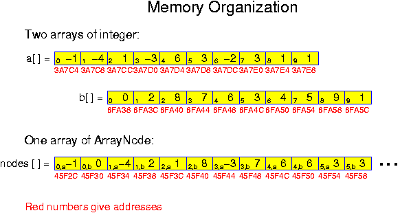
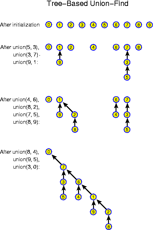
This idea can be realized very simply using an array to represent the set of links:
  void initialize() {
    for (int i = 0; i < n; i++)
      a[i] = i; }

  int find(int k) {
    while (a[k] != k)
      k = a[k];
    return k; }

  void union(int k1, int k2) {
    k1 = find(k1);
    k2 = find(k2);
    if (k1 != k2) // hook k1 to k2
      a[k1] = k2;
Here a root k of a tree is characterized by the fact that it has a[k] ==
k. The good thing is that with the tree-based implementation, there is no need
to access all elements of a set. Thus, there is no need to have the additional
list structure requiring a second array. Conceptually using trees is a step, but
practically it is even easier than the array-based implementation.
How about the efficiency? A find requires that one runs up the tree to find the index of the root. A union, once the two finds have been performed, is trivial, it just requires that one new link is created. So, here we have reduced the cost of the union at the expense of more expensive finds. The finds can actually be arbitrarily expensive: if the tree degenerates, it can have depth close to n. In that case finds may take linear time.

  void initialize() {
    for (int i = 0; i < n; i++)
      a[i] = -1;  }

  int find(int k) {
    while (a[k] >= 0)
      k = a[k];
    return k; }

  void union(int k1, int k2) {
    k1 = find(k1);
    k2 = find(k2);
    if (k1 != k2) {
      if (a[k1] < a[k2]) { // the set of k1 is larger
        int i = k1;
        k1 = k2;
        k2 = i; }
      a[k2] += a[k1];
      a[k1] = k2; } }
Here a root k of a tree is characterized by the fact that it has a[k] <
0. In that case -a[k] gives the size of the tree.
Lemma: A tree of depth k has at least 2^k nodes.
Proof: The proof goes by induction. To settle the base case, we fix that a tree with one node has depth 0. Now assume the claim is correct for given k. How do the depths develop? If T_1 is joined to T_2, and T_1 has depth smaller than T_2, then nothing changes. If T_1 has depth >= the depth of T_2, then the new depth equals the depth of T_1 + 1. While performing unions, new trees of depth k + 1 can thus only arise when a tree T_1 of depth k is joined to another tree T_2, which, because of our clever joining technique, must have at least as many nodes as T_1. Because of our induction assumption, T_1 has at least 2^k nodes, and thus T_1 + T_2 has at least 2^{k + 1} nodes.
Because there are only n nodes in total, this implies that no tree grows deeper than log n.
Corollary: Using trees and performing union-by-size, union takes O(1), while the time for a find is bounded by O(log n).
The given bound is sharp: trees of logarithmic depth may really arise when repeatedly performing union for trees of equal size. If we are mainly interested in limiting the depth of our tree, then we can just as well perform union by depth: the shallower of the two trees (if any) is hooked to the other. Doing this, it is even easier to prove that the number of nodes in a tree with depth k is at least 2^k and that consequently the depth is bounded by log n.
The only further algorithmic idea in this domain is path contraction. That means, that when we are performing find(k), after we have found that find(k) = r, we start once more at k and link all nodes on the path directly to r. This makes the individual finds twice as expensive, but has a very positive impact on the structure of the tree. The idea that expensive operations lead to an improvement of a search structure is not limited to union-find. Similar ideas are also applied for search trees and priority queues. Notice that even a union operation involves two finds, so even a union may lead to changes in the trees more than just hooking one to the other.
Using the same initialize as before, the code for find now looks as follows:
  int find(int k) {
    int l = k;
    while (a[l] >= 0)
      l = a[l];
    // Now l == find(k)
    while (a[k] > 0) {
      int m = a[k];
      a[k] = l;
      k = m; }
    // Now all nodes on the path point to l
    return l; }
Click here
to see the above piece of code integrated in a working Java program. This
program is executing the same example with n = 10 as shown in the pictures.
The idea of path contraction is that we invest something extra right now, in order to exclude that in the future we have to walk this long way again.
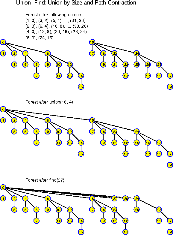
There are alternative implementations of this idea. We can also save the second run, by keeping a trailer and just reducing the depth of the search path by a factor two. This reduces the number of cache misses and will therefore be faster in practice:
  int find(int k) {
    int l = k;
    int m = k;
    while (a[l] >= 0) {
      a[m] = a[l];
      m    = l;
      l    = a[l]; }
    return l; }

  int find(int k) {
    int l = k;
    int m = k;
    while (a[l] >= 0) {
      a[m] = a[l];
      m    = l;
      l    = a[l]; }
    return l; }
The combination of union-by-size (or by height, although the height information may become inaccurate due to the finds) and path contraction leaves very little to desire. The proof of this is skipped, even understanding how good exactly the algorithm is is not trivial.
Theorem:The time for an arbitrary sequence of m unions and finds is bounded by O(m * log^* n).
Here log^*, pronounced log-star, is the function informally defined as "the number of time the log must be applied to reach 1 or less". Thus log^* 1 = 0, log^* 2 = 1, log^* 4 = 2, log^* 16 = 3, log^* 65536 = 4, log^* (2^65536) = 5, etc. In practice this function cannot be distinguished from a constant. And the actual results is even much stronger: the time for any sequence of m >= n unions and finds is bounded by O(m * alpha(n, m)), where alpha(,) is called the inverse Ackermann function. For any m slightly larger than linear, alpha(n, m) is a constant.
It costs very little extra to perform the union by size, but still one may wonder whether it is necessary. Possibly just performing the finds with path contraction might be enough. This makes the union procedure even simpler and faster. Trying examples suggests that this has almost no negative impact on the time of the finds. However, doing this, there is a sequence of n unions and n finds requiring Omega(n * log n) time. This shows that, at least in theory, one really needs the combination of union-by-size and path contraction to obtain the best achievable performance.
Sorting is one of the few problems for which a non-trivial lower bound can be proven relatively easily. We will do this, showing that under reasonable assumption sorting requires at least Omega(n * log n) time. The remarkable thing is that at the same time we know algorithms running in O(n * log n). So, the sorting problem has been solved in the sense that there are optimal algorithms, algorithms whose running time matches the lower bound.
  boolean isSmaller(String s1, String s2) {
    if (s1 == "" && s2 == "") // equal strings
      return false;
    if (s1 == "") // shorter string with common prefix
      return true;
    if (s2 == "") // longer string with common prefix
      return false;
    Char c1 = head(s1); // first character of s1
    Char c2 = head(s2); // first character of s2
    if (c1 == c2) // common first character
      return isSmaller(tail(s1), tail(s2)); // compare remainders
    return c1 < c2; } // compare first character
The lexicographical ordering is not limited to strings. The only typical thing is that strings may have arbitrary length. More generally an ordering can be defined on a product set S_1 x S_2, whenever there is an ordering both on S_1 and on S_2. These do not need to be the same. The ordering relations are denoted "<_1" and "<_2", respectively. The ordering "<" is then defined by (x_1, x_2) < (y_1, y_2) = (x_1 <_1 y_1) or (x_1 == y_1 and x_2 <_2 y_2). If a product of more than two sets S_1 x S_2 x ... x S_n is interpreted as S_1 x (S_2 x ... x S_n), the definition of the lexicographical ordering extends in a natural way.
The objects in the array may be large (for example, records of personal data). Fortunately, this does not need to bother us: an array of objects actually consists of an array of pointers to the objects. Thus, independently of their size two objects can be swapped in constant time:
  if (a[i].key > a[j].key)
  {
    myClass x = a[i];
    a[i]      = a[j];
    a[j]      = x;
  }
Alternatively one might copy all instance variables one-by-one, but for
objects with many instance variables this would be much more expensive.
The most common cost measure is the number of comparisons made. One might also count the number of assignments, but because essentially these cost the same as comparisons, it does not make sense to reduce the number of assignments at the expense of substantially more comparisons.
So, the main goal in this chapter is to find sorting algorithms that minimize the number of comparisons. Only at the end we will encounter a special case which can be solved by counting rather than comparing.
  void sort(int[] a, int n)
  {
    for (int r = 1; r < n; r++)
      for (int i = 0; i < n - r; i++)
        if (a[i] > a[i + 1])
          {
            int x    = a[i];
            a[i]     = a[i + 1];
            a[i + 1] = x;
          }
  }
Click here
to see the above piece of code integrated in a working Java program.
The underlying algorithm is called bubble sort. The name comes from the bubble-like way the elements move through the array. The algorithm is correct because the following invariant property holds:
Lemma: At the end of round r, the last r elements have reached their destination positions.
Proof: The proof goes by induction. For r == 0, it is clearly true. So, assume the statement holds for a given r. Because the last r elements are already positioned correctly and are not addressed any more, they are of no importance: we are just working on the subarray of n - r elements. Consider the maximum m of this subarray. Assume at the beginning of round~r + 1 it is located in a[j]. When i == j, m is exchanged and put at position i + 1. Then i is increased and m is exchanged again. In this way it bubbles until it reaches position n - r - 1 at the end of round r, proving the induction step.
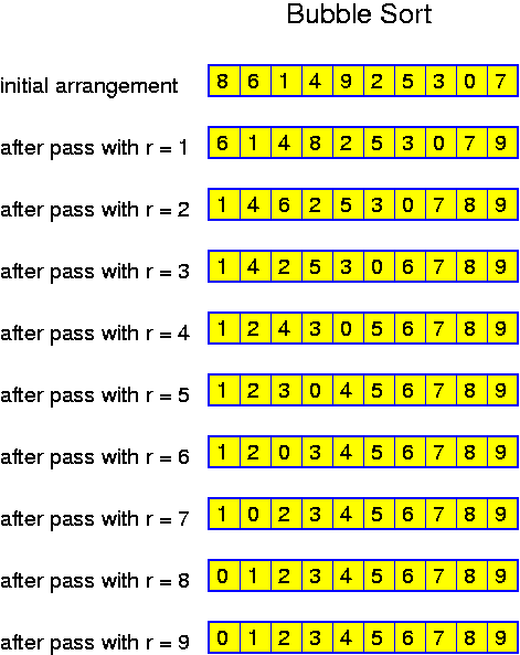
  static int[] merge(int[] a, int[] b)
  {
    int i, j, k, n = a.length + b.length;
    int[] c = new int[n];
    for (i = j = k = 0; k < n; k++)
    {
      if (a[i] <= b[j])
      {
        c[k] = a[i];
        i++;
      }
      else
      {
        c[k] = b[j];
        j++;
      }
    }
    return c;
  }
One has to be careful with the end of the arrays a[] and b[]. In the
current routine we may run beyond it. A handy idea is to add a sentinel:
an element with key infinity at the end of each of them: this will prevent going
beyond the ends because all elements in the array have smaller key values, and
thus these will be written first. As an alternative, one can check again and
again whether i < a.length and j < b.length. Once this is no longer true,
one should copy the possible remainder of a[] or b[] to c[].
Merging takes linear time: the algorithm writes one element for every comparison performed. The last comparison can actually be saved, because as soon as there is only one non-sentinel left, it can be written away without comparison. The operation would be perfect if we would not need the extra space. Theoretically this is not so beautiful, and practically it means that we need memory access to twice as many data. These data must be brought in the cache which takes some extra time. It is quite likely that this time for bringing data in cache dominates the total costs and thus this may take almost twice as long as a comparable routine not requiring additional space. If the merge procedure is called many times, the allocation and deallocation may be expensive too.
  static void merge(int[] a, int b[], int l, int m, int h)
  {
    int i = l, j = m, k = l;
    while (i < m && j < h)
      if (a[i] <= a[j])
        b[k++] = a[i++];
      else
        b[k++] = a[j++];
    while (i < m)
      b[k++] = a[i++];
    while (j < h)
      b[k++] = a[j++];
    for (i = l; i < h; i++)
      a[i] = b[i];
  }

  static void sort(int[] a, int n)
  {
    int[] b = new int[n]; // scratch space
    for (int d = 1; d < n; d *= 2)
    {
      for (int l = 0; l < n; l += 2 * d)
        if (l + 2 * d <= n)
          merge(a, b, l, l + d, l + 2 * d);
        else if (l + d < n)
          merge(a, b, l, l + d, n);
    }
  }
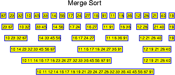
  static void merge(int[] a, int b[], int l, int m, int h)
  {
    int i = l, j = m, k = l;
    while (i < m && j < h)
      if (a[i] <= a[j])
        b[k++] = a[i++];
      else
        b[k++] = a[j++];
    while (i < m)
      b[k++] = a[i++];
    while (j < h)
      b[k++] = a[j++];
  }

  static void sort(int[] a, int n)
  {
    int[] b = new int[n], c; // scratch space and dummy
    int r = 0;
    for (int d = 1; d < n; d *= 2)
    {
      r++;
      for (int l = 0; l < n; l += 2 * d)
        if (l + 2 * d <= n)
          merge(a, b, l, l + d, l + 2 * d);
        else if (l + d < n)
          merge(a, b, l, l + d, n);
        else
          for (int i = l; i < n; i++)
            b[i] = a[i];
      c = a; a = b; b = c; // swap a and b
    }
    if ((r & 1) == 1) // odd number of rounds
      for (int i = 0; i < n; i++)
        b[i] = a[i];
  }
Click here
to see the above piece of code integrated in a working Java program.
The running time in practice depends on two factors: the number of operations performed and the amount of data that must be brought into the cache. The first is closely related to the number of comparisons made, the second is linear in the number of rounds performed. Most likely, it will be profitable to reduce the number of rounds even if this requires extra comparisons (within reasonable limits).
One idea is to start by sorting runs of some well chosen length by an asymptotically slower procedure that is faster for small numbers. Maybe one can find an optimal method for sorting all sequences of 8 elements. Then one saves three passes through the loop. If n = 1024, this means 7 passes instead of 10. In general, this idea reduces the number of rounds by a constant. If the initial sorting is implemented in an optimal way, this does not increase the number of comparisons.
With one comparison we can find the maximum of two elements. With two comparisons we can find the minimum of three elements:
  int minimum(int a, int b, int c)
  {
    if (a <= b)
    // b is not the minimum
    {
      if (a <= c)
        return a;
      return c;
    }
    // a is not the minimum
    if (b <= c)
      return b;
    return c;
  }
This can be used to merge three arrays into one: compare the current
elements of the arrays and write away the smallest. Using this, we can
repeatedly multiply the length of the sorted sequences by three and thus perform
the whole sorting in log_3 n rounds. As log_3 n = log_2 n * ln 2 / ln 3 = 0.63 *
log_2 n, this reduces the number of rounds by a constant factor. The number of
comparisons has increased from about n * log_2 n to 2 * n * log_3 n, which is
larger by a factor 2 * ln 2 / ln 3 = 1.26. This is so little, that it will
certainly be profitable to perform this 3-way merge. One can push further
and apply 4-way or even multi-way merge. In the latter case, the header
elements of the arrays to be merged are inserted in a priority queue and one
repeatedly calls deleteMin().
  void sort(int[] a, int n)
  // sort n elements standing in positions 0, ..., n - 1 of a[]
  {
    if (n > 1)
    {
      int i;
      int a_smaller[n],  a_equal[n],  a_larger[n];
      int n_smaller = 0, n_equal = 0, n_larger = 0;
      int s = a[randomly generated number x, 0 <= x < n];

      // Split the set of elements in three subsets using s
      for (i = 0; i < n; i++)
        if      (a[i] < s)
          a_smaller[n_smaller++] = a[i];
        else if (a[i] == s)
          a_equal[n_equal++] = a[i];
        else
          a_larger[n_larger++] = a[i];

      // Solve two recursive subproblems
      sort(a_smaller, n_smaller);
      sort(a_larger, n_larger);

      // Combine the results
      for (i = 0; i; < n_smaller; i++)
        a[i] = a_smaller[i];
      for (i = 0; i < n_equal; i++)
        a[i + n_smaller] = a_equal[i];
      for (i = 0; i < n_larger; i++)
        a[i + n_smaller + n_equal] = a_larger[i];
    }
  }
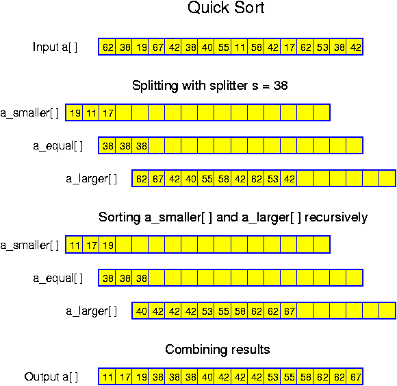
The worst case is that the rank of s lies close to 0 or n. In that case, only a few elements are split off. If this happens again and again, we get a recursion tree of depth Omega(n), and the total running time becomes Theta(n^2).
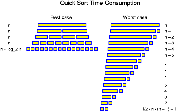
What happens really? Clearly we can not hope to choose medians every time. But, 50% of the selected s are good, in the sense that n/4 < rank(x) < 3/4 n. This probability is independent of n. Every time we are hitting a good splitter, the problem size is reduced by at least a factor 3 / 4. So, the sequence of recursions in which an element x is involved certainly terminates after log_{4/3} n good splitters have been selected from the set to which it belongs. Even the splitters which are not good give some reduction of the problem size, so the expected number of recursive levels in which x is involved is bounded by 2 * log_{4/3} n. Thus, the expected time spent on comparing and rearranging x is O(log n). Because of the so-called "linearity of expectation", the expected time for the whole algorithm equals the sum of the expected times spent for each element. Thus, the expected running time of the quick-sort algorithm is bounded by O(n * log n). A more careful analysis shows that the probability to need substantially more than the expected time is very small.
In practice the most common strategy of this kind is to take "middle of 3" or "middle of 5". It is a good idea to adapt the value of k to n: the larger n, the more one can invest on selecting a good splitter.
Even more so than for merge sort, it is better to no perform the recursion until we have reached a subproblem of size 1: for very small subsets it is rather likely that the division is very uneven. It is much better to apply bubble-sort for all sets with size smaller than some constant m. The optimal choice for m depends on the details of the hardware, but it will not be large. 10 might be reasonable. One can also switch to merge sort: because merge sort is efficient itself, this may be done already for quite large subproblems.
In the case of quicksort a simple modification makes the algorithm in-situ and even saves on the number of elements that are copied. The idea is to not use the additional arrays a_smaller[], a_equal[] and a_larger[], but to swap the elements in the array a[] itself. This can be realized by starting from both sides of the array, searching for elements which stand at the wrong side. If all elements have different values, the splitting may be implemented as shown in the following sorting routine:
  void sort(int[] a, int l, int h, Random random)
  // sort h - l + 1 elements standing in positions l, ..., h of a[]
  {
    if (h > l) // At least two elements
    {
      int low = l;
      int hgh = h;
      int s   = a[random(l, h)]; // choose random element

      // Splitting
      while (low < hgh)
      {
        while (low <= h && a[low] <= s)
          low++;
        while (hgh >= l && a[hgh] >  s)
          hgh--;
        if (low < hgh) // swap a[low] and a[hgh]
        {
          int x = a[low]; a[low] = a[hgh]; a[hgh] = x;
          low++;
          hgh--;
        }
      }

      // Recursion
      sort(a, l, hgh, random);
      sort(a, low, h, random);
    }
The additional tests, low <= h and hgh >= l, are necessary,
otherwise we might run out of the interval if s happens to be the smallest or
largest value in this subarray.
After the splitting, low > hgh and the following holds:
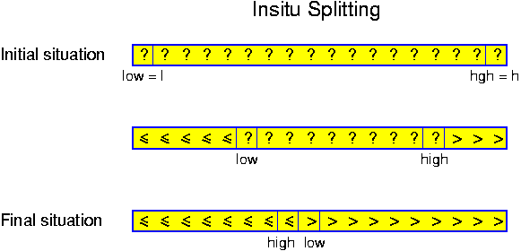
As we have seen, the fourth solution is easy to implement if we use one array for each subset to create, but this is a waste. Even now we would like to perform the sorting in-situ. This is possible, though not as easily as before. It is doubtful whether in practice this is better than the second solution. The idea is to maintain 5 regions instead of 3. There are 4 variables, eql, low, hgh, eqh. At all times eql <= low <= hgh <= eqh. The following properties are maintained invariant:
As long as low < hgh, out of a situation in which the four invariants hold, a new such situation with larger low and/or smaller hgh can be established as follows:
  while (low <= h && a[low] <= s)
  {
    if (a[low] == s)
    {
      int x = a[low]; a[low] = a[eql]; a[eql] = x;
      eql++;
    }
    low++;
  }
  while (hgh >= l && a[hgh] >=  s)
  {
    if (a[hgh] == s)
    {
      int x = a[hgh]; a[hgh] = a[eqr]; a[eqlr = x;
      eqr--;
    }
    hgh--;
  }
  if (low < hgh)
  {
    int x = a[low]; a[low] = a[hgh]; a[hgh] = x;
    low++;
    hgh--;
  }
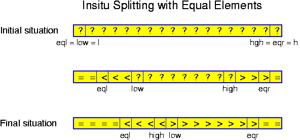
Nevertheless, one might wonder whether O(n * log n) is optimal. For n = 2, one can sort with one comparison. For n = 3, one can find the smallest element with two comparisons, and one more comparison sorts the other two. For n = 4 it already becomes a nice puzzle to just use 5 comparisons. A convenient notation helps: sorting algorithms can concisely be presented by a set of arrows as in the following:
      a   b           a   b   c            a   b   c   d
  1    <->             <->                  <->
  2                    <----->                      <->
  3                        <->              <----->
  4                                             <----->
  5                                             <->
The above shows how to sort 2, 3, 4 numbers with 1, 3, 5 comparisons. Every x <--> y denotes the two elements to compare. If x > x, then the elements are swapped. So, for any input sequence, at the bottom we should find the elements in sorted order, the smallest on the left. The notation with arrows can easily be converted into an algorithm:
  void swap(int[] a, int i, int j) {
    int z = a[i]; a[i] = a[j]; a[j] = z; }

  void sortTwo(int[] a) {
    if (a[0] > a[1]) swap(a, 0, 1); }

  void sortThree(int[] a) {
    if (a[0] > a[1]) swap(a, 0, 1);
    if (a[0] > a[2]) swap(a, 0, 2);
    if (a[1] > a[2]) swap(a, 1, 2); }

  void sortFour(int[] a) {
    if (a[0] > a[1]) swap(a, 0, 1);
    if (a[2] > a[3]) swap(a, 2, 3);
    if (a[0] > a[2]) swap(a, 0, 2);
    if (a[1] > a[3]) swap(a, 1, 3);
    if (a[1] > a[2]) swap(a, 1, 2); }
sortFour() is correct because a[0] holds the minimum after Step 3, because
a[3] holds the maximum after Step 4, and the two middle elements are sorted in
Step 5.
In this case the second approach is more successful: we prove that sorting requires Omega(n * log n) comparisons. For n numbers, there are n! arrangements. Our sorting algorithm must somehow decide which of them corresponds to the current input. We assume that the algorithm is only making comparisons, and is not performing operations on the values. By making a comparison, we can exclude some of the possible arrangements: comparing x = a[i] with y = a[j] either excludes all arrangements with x < y or all arrangements with x > y. So, every comparison gives a certain reduction of the number of possible arrangements. Only once we have reduced the number of possible arrangements to a single one, we may stop and output this single remaining arrangement as the sorted order.
Drawing the set of all possible arrangements at the top and then indicating how, by making comparisons, each of the n! possibilities is singled out gives a tree: In the root represents the set of cardinality n!, the n! leaves the sets of cardinality 1, and the branching in each node is given by the comparisons. This tree is called a decision tree.
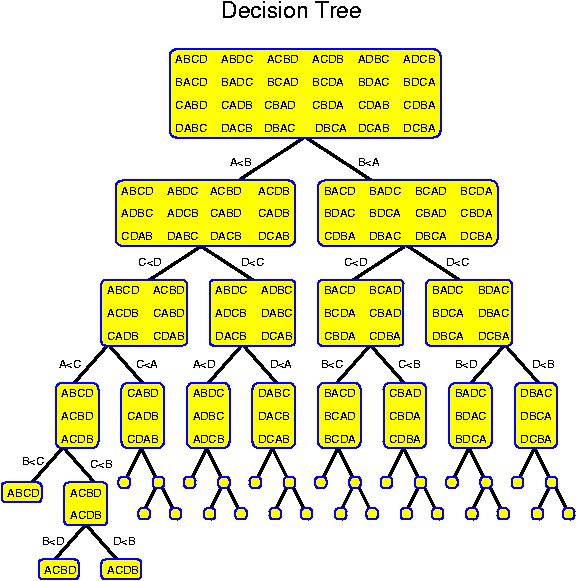
Just like the decision tree, a sorting algorithm is a recipe on how to perform comparisons until only one possible arrangement remains. Actually there is a one-one correspondence between them. Algorithms can readily be turned into trees (though it would be no fun to actually do this for n > 5) and trees can be turned into algorithms with one if-statement for every internal node of the tree. For example, corresponding to the above decision tree we have the following algorithm:
  void sortFour(int A, int B, int C, int D)
  {
    if (A < B)
      if (C < D)
        if (A < C)
          if (B < C)
            printf("The order is ABCD\n");
          else
            if (B < D)
              printf("The order is ACBD\n");
            else
              printf("The order is ACDB\n");
        else
          ...
      else
        if (A < D)
          ...
        else
          ...
    else
      if (C < D)
        if (B < C)
          ...
        else
          ...
      else
        if (B < D)
          ...
        else
          ...
In the case of sorting we are quite happy: the one-one correspondence between comparison-based sorting algorithms and decision trees, makes it much easier to abstract from the details of the algorithms. In the case of sorting it suffices to prove that there is no decision tree of depth smaller than x. Because we are working in a world of binary comparisons, the tree is binary (in the worst case that all keys are different). A decision tree for sorting n elements must have at least n! leaves. We know that a binary tree of depth k has at most 2^k trees. So, for t_n, the minimum number of comparisons for sorting n numbers, we have the following condition
t_n >= round_up(log_2(n!)).
For small values of n, we can use this formula to find t_2 = 1, t_3 = 3, t_4 = 5, t_5 = 7, t_6 = 10. More in general we get:
Theorem: Sorting n numbers requires Omega(n * log n) comparisons.
Proof: n! = Prod_{i = 1}^n i > Prod_{i = n/2}^n i > (n/2)^{n/2}. Thus. log_2 n! > n/2 * (log_2 n - 1) = Omega(n * log n). Stirlings formula can be used to obtain a more accurate estimate: n! ~= (n/e)^n, thus log_2 n! ~= n * log_2(n / e) = n * (log_2 n - log_2 e) ~= n * (log_2 n - 1.44).
So, except for constant factors we now know how many comparisons are needed for sorting n numbers. At first one may believe that in principle one does not need more than round_up(log_2(n!)) comparisons, because a decision tree can always be constructed as follows: at any node choose the comparison that divides the set of remaining possibilities as evenly as possible in two. For all small values of n, this idea leads to trees with the minimal depth of round_up(log_2(n!)). However, for n = 12 this does not work: up(log_2 n!) = 29, and it has been shown that 30 comparisons are necessary (and sufficient) for sorting 12 numbers.
First we consider the special case M == 2. So, all values in a[] are 0 or 1. This is an important special case: for example, the zeroes can stand for personal records of men, the ones for records of women. How should we sort? Quite easy: create two buckets of sufficient size, throw all zeroes in one bucket and all ones in the other. Finally copy all elements back to a[], first the zeroes, then the ones:
  void sort(int[] a, int n)
  // All values in a[] are 0 or 1.
  {
    int[] b0 = new int[n];
    int[] b1 = new int[n];
    int c0 = 0, c1 = 0;

    // Throw ones and zeroes in different buckets
    for (int i = 0; i < n; i++)
      if (a[i] == 0)
      {
        b0[c0] = a[i];
        c0++;
      }
      else
      {
        b1[c1] = a[i];
        c1++;
      }

    // Write all elements back to a[]
    for (int i = 0; i < c0; i++)
      a[i]      = b0[i];
    for (int i = 0; i < c1; i++)
      a[i + c0] = b1[i];
  }
Click here
to see this piece of code integrated in a working Java program. This is
certainly a very fast sorting routine. For n = 10^6 it is 10 times faster then
quick sort!
In the above example and in the following ones, there is a possibly confusing double usage of a[i]. In a comparison like "a[i] == 0", a[i] denotes the key value. In an assignment like "b0[c0] = a[i]", it stands for the object. Only because we are here sorting integers these are the same. In this case the sorting can be simplified even further: it satisfies to count the number c0 of zeroes in a[], and then we can set the first c0 positions to 0 and the remaining ones to 1. But this is cheating: for the sake of simplicity we are considering here how to sort integers, but always we have applications in mind in which these are keys from larger objects.
Suppose now that M is a small constant. How do we extend the above idea? Still simple: create M buckets and throw the elements with value i in bucket i; finally write them back to a[] bucket by bucket. Now it becomes handy to use the key values as indices instead of using a chain of if-statements. So, this is an application of direct addressing.
  void sort(int[] a, int n, int M)
  // All values in a[] are in {0, ..., M - 1}
  {
    int[][] b = new int[M][n];
    int[]   c = new int[M];
    for (int j = 0; j < M; j++)
      c[j] = 0;

    // Throw elements in buckets according to values
    for (int i = 0; i < n; i++)
    {
      int j = a[i]; // key used as index
      b[j][c[j]] = a[i];
      c[j]++;
    }

    // Write all elements back to a[]
    int s = 0;
    for (int j = 0; j < M; j++)
    {
      for (int i = 0; i < c[j]; i++)
        a[i + s] = b[j][i];
      s += c[j];
    }
  }
Click here
to see this piece of code integrated in a working Java program. For M == 2, the
performance is as good as before, but for larger M it deteriorates.
What is worse, is that the algorithm needs n + M + M * n memory. This is acceptable only for very small M. An algorithm is said to be efficient if its consumption of a resource (time or memory) exceeds that of the best solution known by at most a constant factor. In this formal sense the above algorithm is not memory-efficient for M = omega(1), that is, for non-constant M.
The problem of excessive memory usage can be overcome at the expense of some more operations. If we first count the number n_j of elements with value j, 0 <= j < M, then b[j][] can be defined to be of length n_j. Because sum_j n_j = n, this is memory-efficient even for larger M. It is even more efficient to arrange all these buckets after each other in a single array b[]. This leads to the following efficient implementation:
  void sort(int[] a, int n, int M)
  {
    int b[] = new int[n];
    int c[] = new int[M];

    // Count the number of occurrencies of each value
    for (int i = 0; i < M; i++)
      c[i] = 0;
    for (int i = 0; i < n; i++)
      c[a[i]]++;

    // Determine the starting points of the buckets
    int sum = 0;
    for (int i = 1; i < M; i++)
    {
      int dum = c[i];
      c[i] = sum;
      sum += dum;
    }

    // Throw elements in buckets according to values
    for (int i = 0; i < n; i++)
    {
      b[c[a[i]]] = a[i];
      c[a[i]]++;
    }

    // Write all elements back to a[]
    for (int i = 0; i < n; i++)
      a[i] = b[i];
  }
Click here
to see this piece of code integrated in a working Java program. For M == 2, the
performance is even somewhat better than the above versions: saving memory often
goes hand-in-hand with saving time. In C we can save the final copying from a[]
to b[] by passing a[] by reference and instead of the loop making the assignment
*a = b.
The above sorting algorithm is known as bucket sort. Clearly its time and memory consumption is bounded by O(n + M). For all M = O(n) this is memory-efficient. Not a single comparison between elements of a[] is made. Bucket sort does not contradict the proven lower bound, because we very explicitly use the integer-nature of the keys: using direct addressing gives us something like the power of a n-way comparison in constant time.
A disadvantage of bucket sort is that there are quite a lot of operations. More costly is that the memory access in the loop in which the elements are allocated to their buckets is very unstructured. As long as the cache is large enough to hold one cache line for each bucket, this is no big deal, but for large M this causes n cache faults. Therefore, for large M, bucket sort is hardly faster than an optimized version of quick sort.
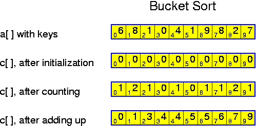
In general, this algorithm can be used to sort numbers in the range 0, ..., M - 1 for M = m^k with k applications of bucket sort, using m buckets in every round, starting with the least significant digits. This requires n + O(m) memory and O(k * (n + m)) time. An important special application is the case that M = n^k, for some constant k. Applying a k-level radix sort with m = n solves the sorting in O(n) time using O(n) memory. This means that sorting can be performed in linear time as long as M is polynomial in n. Theoretically this may be interesting, but practically radix sort is not better than quick sort for M > n^2.
The main disadvantage of bucket sort is that for large M the loop in which the elements are allocated to their buckets causes n cache misses. For the extremely important special case that M == n, this is quite unfortunate. However, if the main memory can accommodate n integers, then on any reasonable system the cache can accommodate sqrt(n) cache lines. So, when applying a two-level radix sort for the special case that M == n, we may assume that m = sqrt(M) cache lines can be accommodated, which implies that the handing-out operations have reasonable cache behavior. In addition this idea reduces the memory consumption from 3 * n to 2 * n + sqrt(n). Comparing the performance of the given bucket sort program with that of the radix sort program, shows that for large n a two-level radix sort is about twice as fast, clearly showing that the sheer number of performed operations is no longer what determines the time consumption.
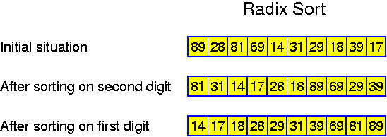
By a subkey we mean one of the keys constituting the entire lexicographical key. If the subkeys lie in a finite range, it may appear natural to use bucket sort again and again. For example, when sorting a set of words, one may start by throwing words in 26 buckets according to their first letters, than splitting the buckets by looking at the second letters, etc. However, one should be aware that bucket sort costs O(M) even if there are very few elements to sort. So, as soon as there are fewer than M elements, another sorting algorithm should be used. Otherwise, when sorting words with five levels of bucket sort, we would create 26^5 buckets, most of them not getting a single word.
Radix sort is different: sorting n numbers up to n^2 - 1, we do not create n^2 buckets at the second level, but only n. At the second (and deeper) level all elements are distributed over one set of buckets again. The advantage is the small number of operations, the disadvantage is that the sorting does not involve ever fewer elements.
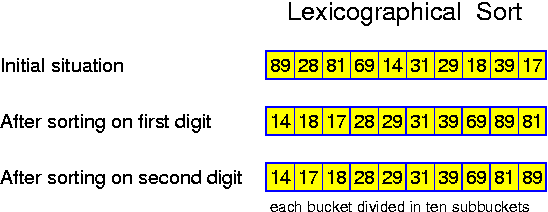
      if (h > l)
        if (h < l + c)
          // Run bubble sort on <= c elements
        else
          // Run quick  sort on >  c elements
Plot the resulting times for c = 1, 2, ..., 20. What is the optimal
choice for c? How much faster is this best variant than the original routine?
A priority queue ADT is a set on which at least the following two operations are supported:
It is also possible to maintain the array sorted. In that case the insertions are expensive, and the deletemins are O(1).
A much better idea is to use a balanced search tree. In that case, the minimum element can be found in logarithmic time, the same as required for inserts (and all other operations). Maintaining an extra pointer to the smallest element (using 2-3 trees this is always the leftmost leaf), the findmin operation can even be performed in O(1) time.
A heap is a tree for which any node v has a key that is smaller (or equal) than the keys of all its children (if any).The above property will be refered to as the heap property. It clearly implies that the smallest occuring key stands in the root of the tree, and that the second smallest element is one of its children. Thus, findmin can be done in O(1): just return the key of the root.
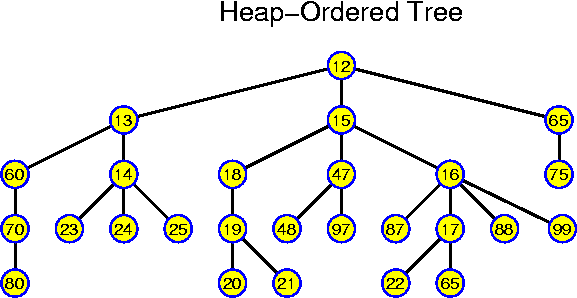
A deleteMin is slightly harder. It is not hard to remove the root, but we should write another element instead of it, so that afterwards the tree is again a heap. But, this is not too hard either. If the root v is deleted, than we may replace it with the smallest of its children. At this level this is correct. In this way the hole that was created by the deletion of v is moved one level down. More generally, the heap property is preserved when we recursively call delete in the following way:
  void delete(node v) {
    if (v has no children) // v is a leaf
      remove v and return;
    else { // v has at least one child
      let w be the child of v with the smallest key;
      set v.key = w.key; // maybe even other data to copy
      delete(w); } }

  int deleteMin(node root) {
    int x = root.key;
    delete(root);
    return x; }
An insert is similar. The new node v can in principle be attached to any node w. If the key of v is smaller than the key of w, then the heap property is restored by exchanging v and w, but possibly v may have to bubble up even further. At a certain level, possibly at the root, v will have found a place in which it is no longer violating the heap property and we are done.
The way the hole is moving through the tree is most commonly called percolation. To be more precise, under insertion the new key is percolating up. In pseudo-code the insertion looks like:
  void percolate_up(node w) {
    if (w has a parent) { // w is not the root
      let v be the parent of w;
      if (v.key > w.key) {
        int x = v.key; v.key = w.key; w.key = x;
        percolate_up(v); } }

  int insert(int x) {
    create a new node w;
    w.key = x;
    attach w to an appropriate node v;
    percolate_up(w); }
From the above, we have seen that one has a lot of freedom for doing things. This will be exploited to come with a very simple and very efficient implementation. The tree will always be kept perfectly balanced: that is, it will always be a binary tree with all levels completely filled, except for possibly the lowest.
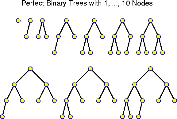
This means, that if we are adding a node, performing insert, we must insert it at the next free place in the lowest level. If the last level is just full, we must create a new level, inserting the element as the left child of the leftmost node in the bottom level.
A deletemin cannot be performed as before, because then we cannot control where the hole is going. Therefore, we are modyfing the routine. The last position in the bottom level is freed, possibly cancelling the whole level. The key v of this node is temptatively placed in the root, and then it percolates down by exchanges with the smaller child. This is slightly more complicated than percolating up. The whole deleteMin now looks like
  void percolate_down(node v) {
    if (v has at least one child) // v is not a leaf
      determine the child w which has smallest key;
      if (key.w < key.v) {
        int x = v.key; v.key = w.key; w.key = x;
        percolate_down(w); } }

  int deleteMin(node root) {
    int x = root.key;
    let w be the leftmost node at the bottom level;
    root.key = w.key;
    remove node w from the tree;
    percolate_down(root);
    return x; }
This procedure is correct: the heap property might only be disturbed along
the processed path, but on any of these positions, finally the root with key
values x, y1, y2 holds the smallest of them.
In this way, the tree has depth bounded by log n (rounded up), so both operations can be performed in O(log n) time. The described delete_min and insert procedures are illustrated in the following picture:
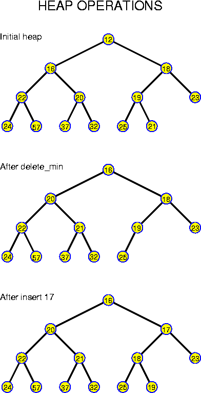
In a really efficient implementation we do not perform exchanges (requiring 3 * pathlength assignments), but have a hole into which the elements are shifted (requiring only 1 * pathlength assignments).
Another observation that is essential for very efficient implementations in practice is that a perfect binary tree can very well be maintained in an array, avoiding all pointers. The idea is to number the nodes level by level from left to right, starting with the root who gets number 0. In that case, for any node with index i, the leftchild has index 2 * i + 1 and the rightchild has index 2 * i + 2. This makes the acces of the children possible by a simple computation, which requires two clockcycles (maybe even one on the average because often additions and multiplications can be executed in parallel), which is negligible in comparison with the cost for a memory access. (If we start with index 1 for the root, then the left child of node i has index 2 * i and the right child 2 * i + 1, which is even simpler to compute). This indexing idea works even for d-ary heaps which are based on perfect d-ary trees.
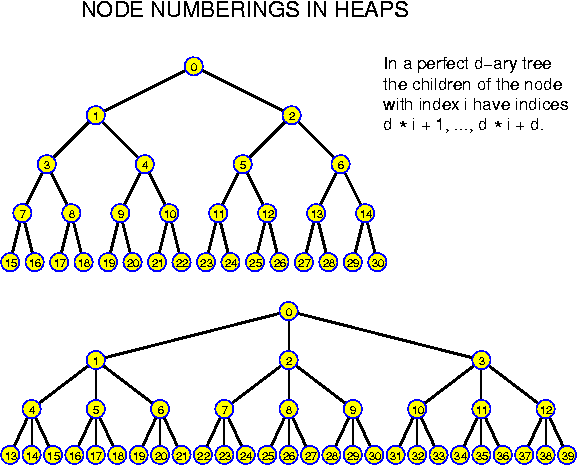
The situation for insertions is different: better. In practice it turns out that insertions go very fast. Much faster than O(log n). The reason is simple, a precise analysis is quite hard. Of course an analysis requires an assumption. Practice cannot be analyzed. So, we assume that the keys are sampled uniformly from an interval, say they are reals in [0, 1]. In the book it is stated that for this case a node moves up only 1.607 levels. Let us try to understand this result.
Consider the case that we are only performing inserts and no deletemin operations. Randomly and uniformly select a key. It is essential that the previous nodes were sampled from the same probability distribution. The node is only moving up k levels, if it is has the smallest key in its subtree of depth k - 1. The lowest level of this tree may have been empty except for the node itself, but all the other levels are full. So, only if the node is the smallest among 2^k or more nodes (also counting the node itself) it is moving up k levels. This means that the expected distance it is moving upwards can be estimated as follows: the probability that the node is moving up exactly k levels is at most 1 / 2^k for all k. Thus we get
E(moveUp) <= sum_{k > 0} k / 2^k = 1 * 1/2 + 2 * 1/4 + 3 * 1/8 + 4 * 1/16 + ... < sum_{i > 0} sqrt(2)^{-i} = 3.414.Here "E(X)" is used to denote the expected value of a random variable X. Remind that E(X) is defined by
E(X) = sum_{all possible values i} i * Probability(X = i).A more accurate estimate is obtained by using
sum_{k > 0} k * a^k = a / (1 - a)^2.Substituting a = 1/2 gives a bound of 2. The precise value is not that important, but one should remember that the expected insertion time is bounded by O(1).
sum_{i = 1}^n log i > sum_{i = n / 2}^n log i > sum_{i = n / 2}^n log (n / 2) = n/2 * (log n - 1) = Omega(n * log n).
Can we hope to do better? Yes. The fact that the expected cost for an insertion is O(1) hints, but not more than that, that we may hope to do it in O(n) time. One idea is to first randomize the input and then perform n times an insert. One can show that the with high probability the whole sequence of insertions costs only O(n) time.
However, this bound can also be established deterministically by a rather simple algorithm. The idea is that we do not maintain a heap at all times (this is not necessary as we are not going to do deletemins during the buildheap). We simply create a perfect binary with n nodes, and then heapify it. That is, we are going to plough through it until everything is ok.
How to proceed? Our strategy must in any case guarantee that the smallest element appears in the root of the tree. This seems to imply that the root must (also) be considered at the end, to guarantee that it is correct. From this observation one might come with the idea that it is a good idea to work level by level bottom up, guaranteeing that after processing level i, all subtrees with a root at level i are heaps. Let us consider the following situation: we have two heaps of depth d - 1, and one extra node with a key x, which connects the two heaps.
                   x
                 /   \
              HEAP1 HEAP2
How can we turn this efficiently into a heap of depth d? This is easy: x
is percolated down.
So, two heaps of depth d - 1 + one extra node can be turned in O(d) time into a heap of depth d. Now, for the whole algorithm we start at level 1 (the leafs being at level 0) and proceed up to level log n:
  // The nodes at level 0 constitute heaps of depth 0
  for (l = 1; l <= round_down(log_2 n); l++)
    for (each node v at level l) do
      percolate_down(v); // Now v is the root of a heap of depth l
    // Now all nodes at level l are the root of a heap of depth l
  // Now the root is the root of a heap of depth round_down(log_2 n)
The correctness immediately follows from the easily checkable claims
(invariants) written as comments within the program, which hold because the
above observation about the effect of percolating down.
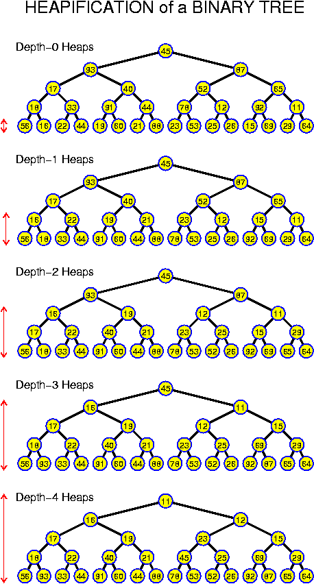
How about the time consumption? At level l we are processing fewer than n / 2^l nodes, and each operation takes O(l) time. Let c be the constant so that time_for_level_l <= c * l, then the total time consumption can be estimated as follows (using the same estimate as above):
sum_{l = 1}^log n c * l * n / 2^l < c * n * sum_{l >= 1} l / 2^l = 2 * c * n. = O(n).
Practically there are reasons to choose d to be a power of two: in that case the array implementation requires only bit shifts for the computation of the location of the parent and the children (and no divisions which might be more expensive). For d-heaps mapping the nodes to consecutive numbers in a way so that the indices of the children can be computed easily is the same as before: start with the root, and number on level by level. Giving number 0 to the root, the children of a node with index i are the nodes with indices d * i + 1, ..., d * i + d.
Denote by f_d(k, i) the index in a perfect d-ary tree at position i of level k (the root being at position (0, 0)). We should prove that the children of node with index f_d(k, i) have indices d * f_d(k, i) + 1, ..., d * f_d(k, i) + d. This can be shown by first analyzing the relation between the indices of the leftmost nodes. f_d(k + 1, 0) = sum_{l = 0}^k d^l = d * sum_{l = 0}^{k - 1} d^l + 1 = d * f_d(k, 0) + 1. Now consider the other nodes. Node f_d(k, i) has index f_d(k, 0) + i and its children have indices f_d(k + 1, 0) + d * i, ..., f_d(k + 1, 0) + d * i + d - 1. Substituting f_d(k + 1, 0) = d * f_d(k, 0) + 1 the result follows.
Choosing a tree of degree d reduces the depth of the tree from log_2 n to log_d n. Thus, a deleteMin now takes O(d * log_d n). This is worse than before. On the other hand, the insert has become cheaper: it only takes O(log_d n). Practically this is not such an interesting improvement as even degree 2 gives us expected time O(1), but theoretically it might be. For example, if we take d = log n, then the cost for the inserts has been reduced to O(log n / loglog n), which is asymptotically faster. If the deleteMin is organized better (for example by using mini heaps at every level) then this kind of constructions give faster insertion without deteriorating the deleteMins.
A more important reason, just as for non-binary search trees, is that every access of a node means a cache or page fault. If the tree is shallow, then the number of these accesses is reduced, which in practice will imply a reduction of the time to perform the operations. The right choice of d depends on the type of application: if each access implies a page fault, then the tree should be kept as flat as possible, and d should be taken very larger (thousands).
A binomial tree has a very special recursively defined structure:
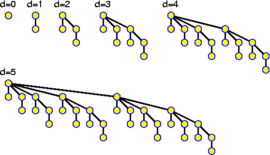
Lemma: A binomial tree of depth d has 2^d nodes.
Proof: The proof goes by induction. The lemma is ok for d = 0 because 2^0 = 1. This is the basis. So, assume the lemma is ok, for all depths up to d - 1. Then, the tree of depth d has 1 + sum_{i = 0}^{d - 1} 2^i = 2^d nodes, because sum_{i = 0}^{d - 1} 2^i = 2^d - 1 (this might again be proven by induction).

With this structure it is very easy to perform a merge. The basic observation is that it is easy to merge two binomial trees of the same depth d - 1 that have the heap property so that the resulting binomail tree of depth d is a heap again: just figure out which of the two roots is smaller, and then attach the other root to this one as a child. The result is a binomial tree because the recursive definition is respected. The result has the heap property because it holds in all non-involved nodes, and because it is preserved for the root of the new tree. Knowing this, two binomial forests can be merged in logarithmic time by playing along the lines of a binary addition: if the number of nodes of the trees have binary representations 10110 and 10111, then in total we have one BNT_0, two BNT_1 which are merged to one BNT_2, this gives us three BNT_2, two of which are merged two one BNT_3 the other remains, then we have 1 BNT_3 which is final, and the 2 BNT_4 are merged to one BNT_5 which is final. So, we get 101101 as representation for the new forest, just as it should be: 45 elements in total. The time is logarithmic, because handling every bit takes O(1) time and there are O(log N) bits.
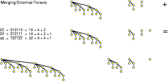
For a deleteMin, we look to the at most log N roots of the binomial trees. The minimum is the minimum of these roots. This minimum element is removed, cutting the concerned tree into several smaller trees. These trees constitute a binomial forest in their own right. It is merged with the rest of the binomial forest to obtain the resulting binomial forest.
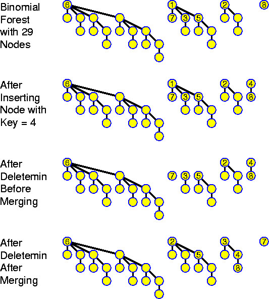
T_exp <= sum_{j >= 0} j / 2^j = 2.
The above result, assumes nothing about the distribution of the keys it only assumes that we have no a priori knowledge about the size N of the binomial forest. Therefore, this is already much stronger than the earlier result for binary heaps, where we needed that the keys were uniformly distributed, a fact which lies outside the influence of the programmer: for certain inputs it is good, for others it is not. In the case of binomial forests we can prove an even somewhat stronger result:
Lemma: For any N, any sequence of M >= log N insertions on a binomial forest with initially N nodes can be performed in O(M) time.
Proof: Above we noticed that an insert on a forest of size N costs
O(z_N) time. Of course, even if z_N = 0 it takes some time. Thus, for a suitable
constant c, the cost of the M insertions is bounded by
T(N, M) = sum_{i = 0}^{M - 1} c * (1 + z_{N + i})
So, in order to prove the lemma,
it suffices to show that sum_{i = 0}^{M - 1} z_{N + i} = O(M) for all N and
sufficiently large M. The numbers z_{N + i} are not so easy to bound: they may
be anything between 0 and log N and fluctuate strongly.
= c * M + c
* sum_{i = 0}^{M - 1} z_{N + i}.
In order to study the phenomenon, we want to exploit an analogy. Consider a person who wants to keep track of his expenses. There are numerous smaller and larger expenses, so this requires quite a considerable bookkeeping and it is likely that some expenses are forgotten. Assume this person has a regular income of 1000 units per month and he had 1270 units on his account at the beginning of the year and 490 units at the end of the year. Then without knowing how much was spent when and where, we can immediately conclude that the sum of all expenses during the year has been 12 * 1000 + 1270 - 490 = 12780.
When trying to determine cost functions in computer science quite often one has to perform "clever bookkeeping". One allocates costs to operations that actually did not really caused them in order to later not have to care when they really arise. This idea is effective here too. Let one_N and one_{N + M} denote the number of ones in the binary expansion of the numbers N and N + M, respectively. Furthermore, observe that for any number X, if we compare the binary expansions of X and X + 1, that any number of ones may have become zeroes and any number of positions may have the same value as before, but that there is exactly one position in which X has a zero where X + 1 has a one. So, let us pay for the creation of ones, rather than for their removal! During the M operations, M zeroes are created. Initially there were one_N, finally there are one_{N + M}, so, sum_{i = 0}^{M - 1} z_{N + i} = M + one_N - one_{N + M} <= M + log N. If M >= log N, this is less than 2 * M.
Thus, ammortizing over at least log N insertions, we obtain O(1) time for the insertions. If we intermix inserts and deletemins, then it may become expensive, because we may go from N = 2^n - 1 to 2^n and back all the time.
Inserts can be performed also directly (this is Exercise 6.35) without relying on the mergeroutine. The idea is that we look for the smallest index j so that b_j = 0 (referring to the binary expansion of N). Then we know that the trees T_0, ..., T_{j - 1} + the new element have to be fused into one new tree with 2^j nodes which is replacing the smaller trees in the binomial forest. One can do this in several ways. One possible way is to add the new element as a new root and then to percolate down. This is correct but not very efficient: at the top level, we have j comparisons, at the next level up to j - 1, and so on. The whole operation takes O(j^2) operations. So, it appears better to nevertheless stick more closely to the merging pattern: first we add 1 to T_0 and create a new tree T'_1, which is added to T_1. This gives a new tree T'_2, which is added to T_2. Etc. This is simple and requires only O(j) time.
A decreaseKey is performed by updating the key and percolating the element up. This takes logarithmic time. An increaseKey is similar: update the key and percolate down. A delete can be performed in several ways. Most efficient appears to be to replace the node by the last leaf which then must be percolated down, analogously to doing a deletemin.
This problem is called the selection problem. Selection can be solved trivially by sorting and then picking the right element. If the numbers do not allow a fast linear-time sorting method, then this is not a good method because of the O(N * log N) time consumption.
Another simple method is to perform k rounds of bubble-sort (in a variant that makes the smallest numbers reach their positions first) and then take the number at position k. This costs O(k * N), which is good for small k, but worse than O(N * log N) for large k.
The same time is obtained when generalizing the idea to find the minimum: a pocket with the currently smallest k numbers is maintained. Each new number to consider is compared with these k and if it is smaller then the largest one, this largest one is kicked out. This idea, however, can be improved: using a heap with the largest element in the root with k elements, the largest element can be found in constant time, and replacing it (followed by a percolate-down) takes O(log k) time. Thus, this reduces the time to O(N * log k), which is less than O(N * log N) for a somewhat larger range of k.
A simple alternative is to apply buildHeap to all N elements, building a heap in O(N) time, and then perform k deleteMins. This has the same complexity. This idea can be improved further: there is no need to really delete the elements from the heap. The algorithm can also search from the root for the k smallest elements. The crucial observation is that an element with rank i + 1 is a neighbor of one of the elements with ranks i or less. From among these elements, it is the one with smallest value. Thus, the problem of finding the element with rank k (and all other elements with smaller ranks) can be solved by a special kind of search through the tree:
  /* The heap is called H */
  Create an empty priority queue Q;
  Insert the key of the root into Q;
  for (i = 1; i < k and Q not empty; i++) {
    x = Q.deleteMin(); /* x has rank i */
    let p be the node of H from which x is the key value;
    if (p has a left child)
      insert the key of the left child into Q;
    if (p has a right child)
      insert the key of the right child into Q; }
  if (Q is empty)
    return some_special_value_flagging_error;
  else
    return Q.deleteMin();
This routine (given the already created heap H) costs O(k * log
maximum_size_of_Q). Because every step netto adds at most one node to Q (the key
of node p is removed and at most two new keys are added), maximum_size_of_Q
<= k, and therefore this operation runs in O(k * log k), independently of the
size of the heap!
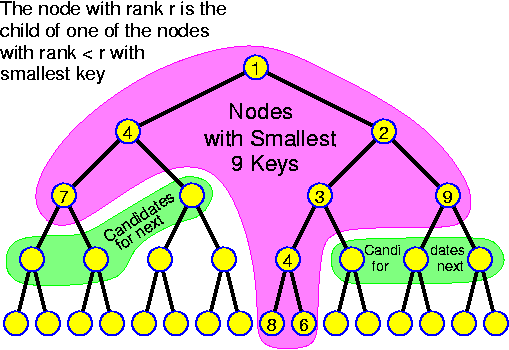
This last idea may be interesting if a heap is given, but if the input is an array with n numbers without any structure, then there are deterministic and randomized algorithms for performing selection in O(N) time, which are simpler and more efficient.
An advantage of heap sorting is that the answer is produced gradually. If we use a heap and call buildHeap first, then after O(n + k * log n) time the first k elements are available. Using quick sort, no output is avaliable until shortly before the end. Of the discussed sorting methods, only bucket sort shares this property, but its efficiency is far worse. So, if the sorted sequence is the input to a follow-up routine, then applying heap sort allows to pipeline the two operations.
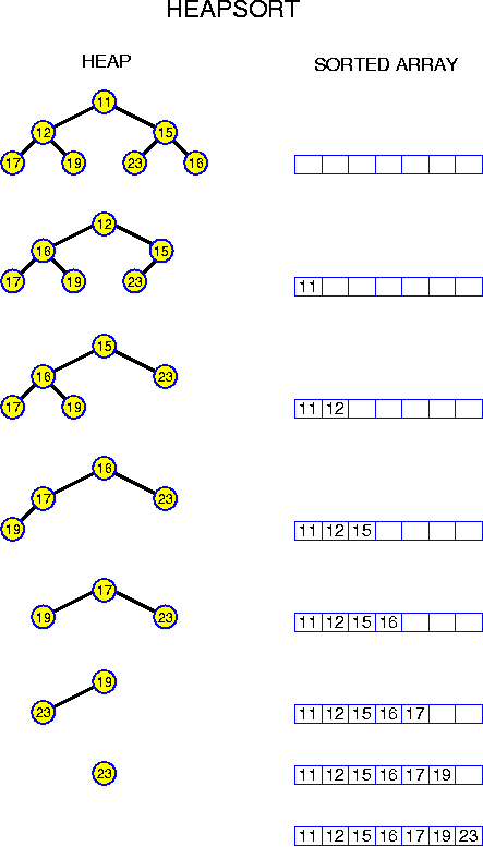
One might have thought that constructing a heap is closely related to sorting, but the above shows that it is actually much less. It is much closer related to finding the minimum.
Let T_1 be the time for the operation insert and T_2 be the time for deleteMin. Considering the above and the lower bound on sorting, prove a lower bound on T_1 + T_2 when we are handling n elements in total.
Assume there is also a method buidlQueue. Outline a sorting algorithm using this method. Let T_3(n) be the time for building a priority queue of n elements. derive a lower bound on a combination of T_1 and T_3(n).
In connection with graphs there are many notions. Some of them are important already now. A neighbor of a node u is any node v for which there is an edge (u, v). In this case one also says that v is adjacent to u. The nodes u and v are called the endpoints of the edge. A path from u to w is a sequence of edges (u, v_1), (v_1, v_2), ..., (v_{k - 1}, w) connecting u with w. A path is called simple if edges are used at most once. A cycle is a simple path which has the same begin- and endpoint. In the example this means that u == w. A graph without cycles is called acyclic. A tree is an acyclic and connected graph. By extension are directed graphs called trees when it is a tree considered as an undirected graph, and when all edges are directed towards or away from a specific node called root. A forest is a set of trees. The length of a path is the number of used edges, in the example the path has length k. The distance from u to v is the length of the shortest path between u and v. A graph is called connected if any pair of nodes u, v there is a path running from u to v. For directed graphs one mostly speaks of strongly connected if we take the direction of the edges into account for these paths, otherwise one speaks of weakly connected. A connected component is a maximum subset of the nodes that is connected. For directed graphs one speaks of strongly (weakly) connected components. A spanning tree is a tree that reaches all nodes of a connected graph. A spanning forest is a set of trees, one for each connected component of a graph. The degree of a node u is the number of edges with endpoint u. The degree of the graph is the maximum of the degrees of all nodes. The number of nodes is often denoted n, the number of edges m. If m = O(n) (as in road graphs), then the graph is said to be sparse. If m is much larger than linear (but as long as there are no multiple edges m = O(n^2)), the graph is called dense. If an edge (u, v) occurs more than once (that is, the "set" of edges is actually a multiset), then we will say that there are multiple edges. A graph without multiple edges is said to be simple. A self-loop is an edge (u, u). It is common to require that graphs are simple without self-loops. Such graphs have at most n * (n - 1) edges if they are directed and at most n * (n - 1) / 2 edges if they are undirected.
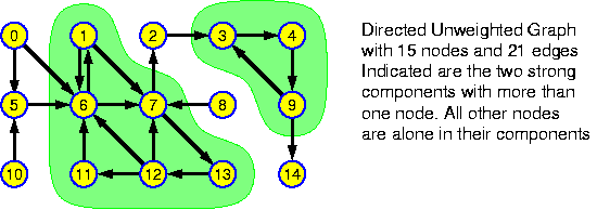
A very easy way to represent graphs in the computer is by creating for each node a set of all its neighbors. This is a particularly good idea for sparse graphs. In general one might use linear lists for these sets. This is called the adjacency list representation of the graph. If all edges have about the same degree with a maximum g, then it is much more convenient to represent the graph as an array of arrays of length g, storing for each node its degree as well. For dense graphs the most appropriate representation is as an adjacency matrix: an n x n boolean matrix, where a 1 at position (u, v) indicates that there is an edge (u, v). If the graph is undirected, the adjacency matrix is symmetric.
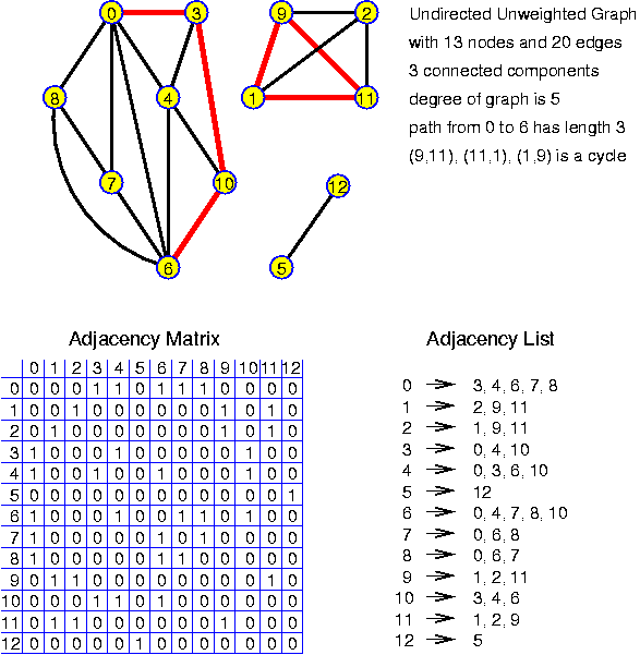
  void BFS_Numbers(int[] bfs_numbers) {
    for (v = 0; v < n; v++)
      visited[v] = false;
    counter = -1;
    create an empty queue Q;
    for (r = 0; r < n; r++)
      if (not visited[r]) { /* r is the root of a new component */
        counter++;
        bfs_number[r] = counter;
        enqueue r in Q;
        visited[r] = true;
        while (Q not empty) {
          dequeue first element from Q and assign it to v;
          for (each neighbor w of v)
            if (not visited[w]) { /* new unvisited node */
              counter++;
              bfs_number[w] = counter;
              enqueue w in Q;
              visited[w] = true; } } } }
Clearly every node is numbered only once, because only nodes that were unvisited are assigned a value. Because counter is increased just before numbering a node and never decreased, all numbers are different.
All nodes are enqueued exactly once, and upon dequeuing all there outgoing edges are considered. This means that the algorithm has running time O(n + m).
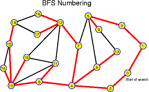
  void DFS_Numbers(int[] dfs_numbers) {
    for (v = 0; v < n; v++)
      visited[v] = false;
    counter = -1;
    create an empty stack S;
    for (r = 0; r < n; r++)
      if (not visited[r]) { /* r is the root of a new component */
        push u on S;
        while (S not empty) {
          pop first element from S and assign it to v;
          if (not visited[v]) { /* New unvisited node */
            visited[v] = true;
            counter++;
            dfs_number[v] = counter;
            for (each neighbor w of v)
              push w on S; } } } }
As before this algorithm numbers each node only once with different numbers from 0 to n - 1. Here the nodes are declared visited only after they are popped from the stack. This implies that nodes may be pushed on the stack many times, and that the size of the stack may become as large as m (even 2 * m for undirected graphs). This is not such a large disadvantage: the graph itself also requires so much storage. If one nevertheless wants to prevent this, one should either apply the recursive algorithm, where the command "push w on S" is replaced by a conditional recursive call to the DFS procedure, or one should push instead of just w also v, and the index of w within the adjacency list of v. When popping this entry w, the next neighbor of v should be written instead of it.
  void dfs(int v, int* pre_counter, int post_counter,
         int[] pre_number, int[] post_number, boolean[] visited) {
    visited[v] = true;
    (*pre_counter)++;
    pre_number[v] = *pre_counter; /* preorder number */
    for (each neighbor w of v)
      if (not visited[w])
        dfs(w, counter, dfs_number, visited);
    (*post_counter)++;
    post_number[v] = *post_counter; /* postorder number */ }

  void dfs_caller(int dfs_number) {
    for (v = 0; v < n; v++)
      visited[v] = false;
    pre_counter = post_counter = -1;
    for (r = 0; r < n; r++)
      if (not visited[r])
        dfs(r, &pre_counter, &post_counter,
          pre_number, post_number, visited); }
Here we computed two types of numbers: preorder DFS numbers and postorder DFS numbers depending on whether they were assigned before or after the recursion. The preorder numbers are the same that were just called "dfs numbers" before. The importance of computing both types of numbers will become clear soon.
The program is written C-like. In Java where integer parameters cannot be passed by reference, one should either make counter global (ugly but efficient), or pass it in some kind of object, for example as an object from the class "Integer".
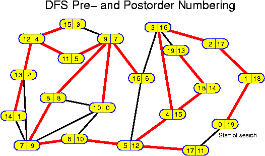
  void Connected_Components(int[] component) {
    for (v = 0; v < n; v++)
      visited[v] = false;
    create an empty queue Q;
    for (r = 0; r < n; r++)
      if (not visited[r]) { /* r is the root of a new component */
        component[r] = r;
        enqueue r in Q;
        visited[r] = true;
        while (Q not empty) {
          dequeue first element from Q and assign it to v;
          for (each neighbor w of v)
            if (not visited[w]) { /* new unvisited node */
              component[w] = r;
              enqueue w in Q;
              visited[w] = true; } } } }
Hereafter, for all nodes v, component[v] gives the index of the "root" of
the component. In this case, this index equals the smallest index of the nodes
belonging to the component. The graph is connected if and only if component[v] =
0 for all v.
The DFS algorithm can be used to determine the connected components in the same way as the BFS algorithm.
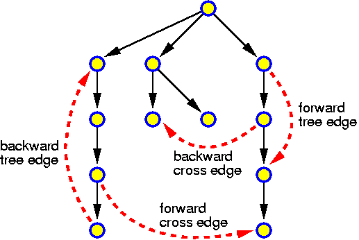
With respect to a given tree (for example the DFS tree of a graph) for which we have computed pre- and postorder numbers, edges can be classified in constant time per edge as follows:
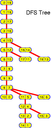
For undirected graphs this gives a particularly easy test for cycles: a minimal modification of the DFS algorithm satisifes. For example, in the recursive algorithm the fragment
      if (not visited[w])
        dfs(w, counter, dfs_number, visited);
can be replaced by if (not visited[w])
dfs(w, counter, dfs_number, visited);
else
printf("Edge (" + v + ", " + w + ") closes a cycle!\n");
For directed graphs, this may detect false cycles: backward cross edges and forward tree edges lead back to earlier visited nodes but do not give cycles (for undirected graphs this is no problem because there is no distinction between backward and forward tree edges, while backward cross edges do not exist). However, these can easily be distinguished from backward tree edges. We need one extra boolean variable for marking nodes for which the recursion is finished. The whole algorithm then looks as follows:
  void cycle_test(int v, boolean[] started, boolean[] finished) {
    started[v] = true;
    for (each neighbor w of v)
      if (not started[w])
        cycle_test(w, started, finished);
      else
        if (not finished[w]) /* (v, w) is a backward tree edge */
          printf("Edge (" + v + ", " + w + ") closes a cycle!\n");
    finished[v] = true;

  void cycle_test_caller() {
    for (v = 0; v < n; v++)
      started[v] = finished[v] = false;
    for (r = 0; r < n; r++)
      if (not started[r])
        cycle_test(r, started, finished); }
  void Unweighted_SSSP(int s, int[] distance) {
    for (v = 0; v < n; v++)
      distance[v] = infinity;
    create an empty queue Q;
    distance[s] = 0;
    enqueue s in Q;
    while (Q not empty) {
      dequeue first element from Q and assign it to v;
      for (each neighbor w of v)
        if (distance[w] == infinity) { /* new unvisited node */
          distance[w] = distance[v] + 1;
          enqueue w in Q; } } }
The algorithm is so that nodes v that are unreachable from s because they
lie in another component have distance[v] = infinity, which appears to be
reasonable.
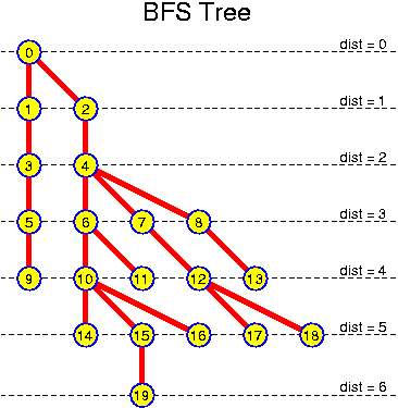
Clearly this computes upper bounds on the distances, because by induction over the time we may assume that all times distance[v] >= distance(s, t), using the triangle inequality which states that for all nodes
distance(s, w) <= distance(s, v) + distance(v, w).Here distance(u, v) denotes the real distance in the graph from node u to node v. It is not so easy to prove the (rather obvious) fact that Unweighted_SSSP computes the correct values:
Lemma: The values of distance[v] for the nodes that are enqueued (dequeued) is monotonically increasing.
Proof: Assume that this is true until step t. Then, in step t we are dequeuing a node v with distance[v] >= distance[v'] for all nodes that were dequeued previously. Here we essentially use that in a queue nodes that were enqueued earlier are also dequeued earlier (the FIFO order). Thus, the largest distance value of the nodes on the queue is at most distance[v] + 1, the distance value of the newly enqueued elements, so the property is maintained.
Theorem: The values of distance[v] are correct.
Proof: It remains to show that the distances are not too large. The proof goes by contradiction. Assume that distancce[w] > distance(s, w) for some w, and assume that w is the node with smallest distance(s, w) which gets assigned a too large value distance[w]. Let u be the last node before w on a shortest path from s to v. distance(s, w) = distance(s, u) + 1. Because u lies closer to s than w, we may assume that distance[u] = distance(s, u). Let v be the node which was responsable for enqueuing w. distance[w] = distance[v] + 1. Because distance[v] + 1 = distance[w] > distance(s, w) = distance(s, u) + 1 = distance[u] + 1, it follows that distance[v] > distance[u]. Thus, according to the previous lemma, node u will be dequeued before node v. Thus, w should have been enqueued by u instead of v, and we should have distance[w] = distance[u] + 1. This is a contradiction, which can be traced back to our assumption that there is a node w with distance(s, w) < distance[w].
In this kind of proofs it is very common to argue by contradiction, focussing on a supposed first occasion for which the algorithm makes a mistake. If there is no first mistake, then there is no mistake at all! void Positively_Weighted_SSSP(int s, int[] distance, int[][] weight) {
for (v = 0; v < n; v++)
distance[v] = infinity;
create an empty priority queue PQ;
distance[s] = 0;
enqueue s in PQ with priority 0;
while (PQ not empty) {
perform a deleteMin on PQ and assign the returned value to v;
for (each neighbor w of v) {
d = distance[v] + weight[v, w];
if (distance[w] == infinity) { /* new unvisited node */
distance[w] = d;
enqueue w in PQ with priority d; }
else if (d < distance[w]) { /* new shorter path */
distance[w] = d;
decrease the priority of w in PQ to d; } } } }
At most n elements are enqueued and dequeued. At most m decreasekey operations are performed. It depends on the priority queue used how much time this takes. Using a normal heap plus some way to find specified elements, all operations can be performed in at most O(log n) time, so O((n + m) * log n) in total. Better priority queues (Fibonacci heaps) allow to perform the decreasekey operations in O(1) time, using these Dijkstra's algorithm runs in O(m + n * log n).
The proof of correctness of the algorithm is similar to the proof of correctness for the unweighted case. First one shows that the nodes that are dequeued have increasing distances.
Lemma: The values of distance[v] for the nodes that are dequeued is monotonically increasing.
Proof: Assume that this is true until step t. Then, consider the node w dequeued in step t. Let v be any node dequeued before. If both nodes were on the queue when v was dequeued using deletemin then distance[v] <= distance[w]. If w was added or updated after v was deleted, then distance[w] = distance[v'] + weight[v', w] for some node v' which was dequeued after v, and which by the induction assumption has distance[v'] >= distance[v]. But then, distance[w] >= distance[v] + weight[v', w] >= distance[v]. It is at this point that we essentially use that weight[v', w] >= 0. Otherwise this lemma cannot be proven!
Theorem: The values of distance[v] are correct.
Proof: As before it can be shown that the values of distance[] at all times give an upper bound on the distances: as long as they are infinity, this is clear, once they have a finite value, the value corresponds to the length of a path: there may be shorter paths, but this path can be used for sure. So, assume that distance[v] >= dist(s, v) for all nodes at all times. Consider the node w lying closest to s, having smallest value of dist(s, w), that upon dequeuing has distance[w] > dist(s, w). Let v be the last node before w on a shortest path from s to w. Thus, dist(s, w) = dist(s, v) + weight[v, w]. Because weight[v, w] > 0, we have dist(s, v) < dist(s, w), and thus v gets correct value distance[v] = dist(s, v), because of our assumption that w is the node closest to s with too large distance[] value, we have distance[v] = dist(s, v) < dist(s, w) < distance[w], and therefore, because of the previous lemma, v will be dequeued before w. But at that occasion the algorithm would have set distance[w] = distance[v] + weight[v, w] = dist(s, v) + weight[v, w] = dist(s, w), in contradiction with the assumption that distance[w] > dist[s, v].
In the following picture the action of Dijkstra's algorithm is illustrated. Edge weights are indicated along the edges, the current values of distance[] are indicated in the nodes. 99 stands for infinity. Nodes that have been removed from PQ have final distance value. The (connected) subgraph with these nodes is marked.
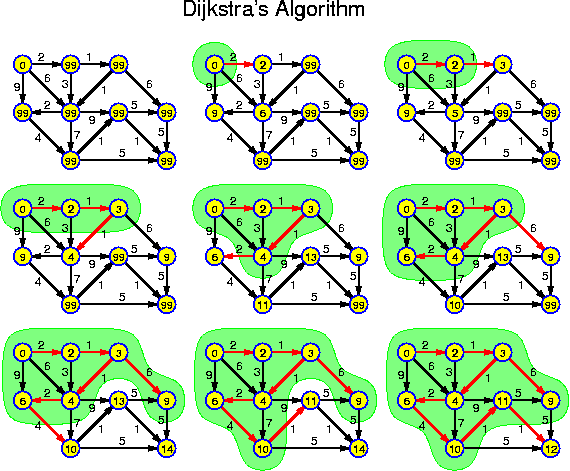

Fortunately, there are several simple solutions. Unfortunately, these algorithms are considerably slower. One is known under the name "Floyd-Warshall Algorithm" and has running time O(n^3). Because of its simplicity and the very small constants hidden in the O(), this algorithm is nevertheless rather practical. It actually solves the all-pairs-shortest-path problem. If this is what one needs, it is a good option. Another algorithm, much closer to Dijkstra's is called the "Bellman-Ford algorithm". The only data structure it needs is a queue (not a priority queue). It solves the SSSP problem in O(n * m). For sparse graphs this is quite ok, for dense graphs Floyd-Warshall may be better.
In general, the notion of shortest paths is not well-defined when there are so-called negative-cost cycles, cycles on which the sum of all costs is negative (or zero). One must either assume that no such cycles exist (that is what we will do in the following), or one must have a mechanism for detecting them.
  void Negatively_Weighted_SSSP(int s, int[] distance, int[][] weight) {
    /* There should be no negative-cost cycles! */
    for (v = 0; v < n; v++)
      distance[v] = infinity;
    create an empty queue Q;
    distance[s] = 0;
    enqueue s in Q;
    while (Q not empty) {
      perform a dequeue on Q and assign the returned value to v;
      for (each neighbor w of v) {
        d = distance[v] + weight[v, w];
        if (d < distance[w]) { /* new shorter path */
          distance[w] = d;
          if (w not in Q)
            enqueue w in Q; } } } }
This algorithm is really very simple, but also quite dumb: all nodes on
the queue are dequeued, processed and possibly enqueued again and again.
Nevertheless, there are no substantially better algorithms. Does the algorithm
terminate at all? Yes, if there are no negative cycles. How long does it take to
terminate? For this analysis we need to introduce the concept of a round:
round 0 consists of processing s, round r > 0 consists of processing all
nodes enqueued in round r - 1. The time analysis is based on
Lemma: In round r there are at most n - r nodes on the queue.
Proof: The lemma follows once we have shown that in round r all nodes whose shortest path from s goes over at most r edges have reached there final distance and will therefore not be enqueued again. The proof goes by induction. For r = 0, the claim trivially holds: s has reached its final distance (we use that there are no negative-cost cycles). Now assume it holds for r - 1. Consider a node w whose shortest path from s goes over r edges. Let v be the last node on this path before w. v has reached its final distance in round r' <= r - 1. When v was getting its final distance, it was enqueued a last time, and in round r' + 1 <= r the algorithm sets distance[w] = distance[v] + c[v, w], which is the correct value. So, every round at least one node will not reappear in the queue anymore.
The lemma implies that there are at most n rounds. As in every round at most m edges must be processed, we get the following theorem, which gives a rather pessimistic view. In practice there will often be fewer rounds and for those graphs that require many rounds, typically one has not to process all edges every time.Theorem The Bellman-Ford algorithm has running time O(n * m).
In the following picture the operation of the Bellman-Ford algorithm is illustrated. Because the order in which the neighbors of a node is not part of the specification of the algorithm, there are various correct possibilities, the picture shows one of them. The marked nodes are those that are not in the queue at the beginning of this stage and will not appear in the queue anymore.
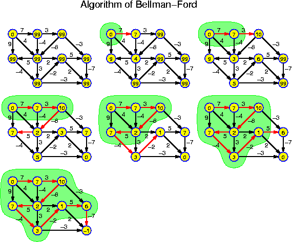
  void Find_Shortest_Path_Tree(int[] distance, int[][] weight,
        int predecessor[]) {
  /* distance[] gives the distances from node s */
  for (all nodes w)
    predecessor[w] = w;
  for (all edges (v, w))
    if (distance[v] + weight[v, w] == distance[w])
      predecessor[w] = v; }
The routine is given for directed graphs. For undirected graphs (depending on the input format) it may be necessary to consider an edge (v, w) both for w and for v. In the current version predecessor[w] may be set several times if there are several paths of the same length. This may be prevented by performing the assignment only when predecessor[w] == w, but this does not make the routine faster.
This routine takes O(n + m) time independently of the type of graph, so these costs are negligible except for unweighted graphs. For weighted graphs it will certainly be more efficient to determine the edges by a separate procedure. But, even for unweighted graphs it may be profitable to perform a second pass over all edges: this reduces the amount of data that are handled in a single subroutine, and may therefore allow to hold a larger fraction of the graph in cache.
Afterwards every node has a unique predecessor, and the graph defined by predecessor[] is acyclic: otherwise there would be a zero-cost cycle. So, the whole graph defined by predecessor[] constitutes a tree directed towards s, spanning all nodes reachable from s. In particular: independently of m, the set of all shortest paths has size n.
Fact: A graph has an Euler tour if and only if all nodes have even degree. A graph has an Euler path if exactly two nodes have odd degree.
The positive side of this claim will follow from the construction hereafter. the negative side is not hard to prove. First we reduce the Euler path problem to the Euler tour problem: if v_1 and v_2 are the two nodes with odd degree, then we can add a single extra edge (v_1, v_2). Now all nodes have ecven degree. Construct a tour for this graph, and start the tour in v_1 first traversing the edge (v_2, v_1) (if the tour runs the other direction, then one starts with (v_1, v_2) or one can reverse the tour). This tour finishes in v_1 again. Omitting the first edge of the cycle gives a path running from v_1 to v_2.
How to construct a tour? The algorithm is simple:
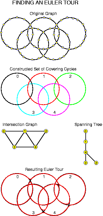
Another important application is as a subroutine in a slightly more advanced problem. Consider a group of friends who have rented a fittness center for two hours. There are n_1 friends and n_2 training machines. Each of them wants to train for 30 minutes on 4 (not necessarily different) machines. Two questions arise:
There is a big difference between these questions. The first is a question about existence. So far we were not confronted with existence questions. Clearly the smallest element in a set can be selected, clearly a sorted order can be constructed, clearly membership can be tested, and elementary algorithms are obvious. For our problem it is not a priori clear that there exists any solution. Maybe we are just asking too much.
The second question is of a different nature. Here we ask about computability. Proving existence might for example go by contradiction and does not need to be constructive. Clearly any construction implies existence, but the other implication does not hold, and there are many problems for which we know that a solution exists, but for which so far no one could give an algorithm with acceptable (= less than exponential) running time.
Fortunately, in the case of the fittness center, there is a surprisingly simple algorithm. It is based on our accumulated knowledge. If there are more than four persons wanting to use the same machine, than clearly they cannot be scheduled in 4 time slots. So, in that case the answer to the first question is negative. Therefore, in the remainder of the discussion, we assume that there are at most four persons wanting to use any of the machines.
We first abstract the problem, reformulating it as a problem for graphs. There is a node for each of the friends and a node for each of the machines. There is an edge for each of the wishes. That is, if person i wants to use machine j, there is an edge (i, j). This graph is bipartite: all edges run between the subset V_1 of n_1 nodes corresponding to the friends and the subset V_2 of n_2 nodes corresponding to the machines.
This graph has degree 4 (each person wants to train on four machines, each machine is selected at most four times). If we succeed to allocate a number from {0, 1, 2, 3} to all edges so that for each node of V_1 and V_2 no two edges have the same number we are done. An assignment of a value x to edge (i, j) can namely be viewed as an assigning person i to machine j in time slot x. The condition that all nodes in V_1 and V_2 get each number at most once means that a person is not scheduled to more than one machine at a time and that a machine is not allocated to more than one person at a time. Assigning values from {0, 1, 2, 3} is equivalent to coloring the edges with four different colors. Therefore, the problem we are considering is known under the name minimum bipartite graph coloring.
Several "greedy" strategies do not work. A first idea is to start allocating the colors to the first node of V_1, then the second and so on. When assigning the colors of node i, we should respect the conditions imposed by earlier assigned colors. If one is lucky this may work, but in general this approach will get stuck when we must assign a color c to an edge (i, j) while node j has an edge (i', j) for some i' < i, which was already assigned color c while coloring node i'. Another "greedy" strategy may also work, but not always. The idea is that one tries to assign the colors one by one. The algorithm gets stuck when, while assigning color c, one comes to a node i for which all the uncolored edges lead to nodes which already have an edge that was given color c before.
The bipartite graph coloring problem can be solved in several ways. The most obvious is to improve the color-by-color approach. This leads to a correct but inefficient algorithm, having running time O(g * sqrt(n) * m), where g is the degree of the graph. It is much better to apply an algorithm based on finding Euler tours (where we do not care about getting several cycles, as long as all edges are covered exactly once). For the special case of a graph with degree 4, the idea is to find a Euler tour (it was no coincidence that the example considers a graph of degree 4 and not 5). The edges on this tour are then numbered alternatingly 0 and 2. Notice that for each node of V_1 and V_2 there are exactly two edges with each number: the edges on the tour leading into the nodes of V_1 get one number and the edges leading into the nodes of V_2 get the other number. So, we have constructed two bipartite subgraphs of degree 2. For these we repeat the procedure. Allocating 1 to half of the edges that previously had 0 and 3 to half of the edges that previously had 2.
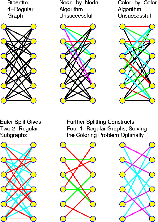
In general, for a graph of degree g = 2^k, the algorithm consists of k rounds. In round i, 0 <= i < k, the algorithm is working on 2^i subgraphs in which all nodes have degree 2^{k - i}. Each of the 2^i operations in round i takes O(n + m_i) = O(n + 2^{k - i} * n) = O(2^{k - i} * n) time, so the total amount of work in any of the rounds is O(2^k * n) = O(m). Thus, in total over all rounds the algorithm takes O(k * m) time. A famous theorem from graph theory (known as "Hall's" or "König's" theorem) states that any bipartite graph with degree g can be colored using only g different colors: a positive answer to the existence question. However, for g which are not powers of 2, the construction of such colorings is considerably harder: the problem of computability. But, after much research, concluded in 2001!, it has been established that even the general case can be solved in O(k * m) time, where k = log g, g being the degree of the graph.
If the forest should be light, why not start with the lightest edge? This we may repeat. So, the idea is to do the following:
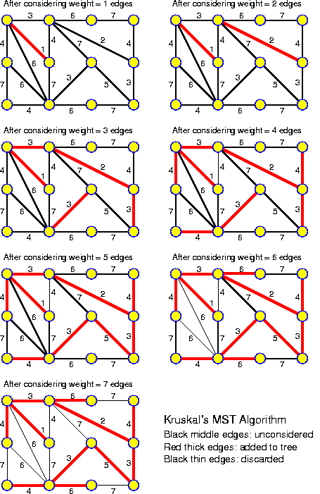
Lemma: F is a spanning forest.
Proof: The proof goes by contradiction, We assume that in F there are nodes in the same connected component of the graph, which are not connected by a path in F. Let C_u be the set of nodes reachable from u by nodes in F. Consider a path from u to v. Because v not in C_u, there must be two nodes u' and v' on this path, connected by an edge (u', v'), with u' in C_u and v' not in C_u. At some step of the algorithm, the edge (u', v') was considered. The only reason why it may not have been added to F is that u' and v' already were connected by a path in F. But because edges are never removed from F, this implies that u' and v' are connected by a path in F at the end of the algorithm, contradicting the fact that v' not in C_u.
Lemma: F is a minimum-weight spanning forest.
Proof: For the proof we need the concept of a promising subset. A subset of the edges is called promising (other names are in use as well), when there is a minimum spanning forest containing these edges. The empty set is promising. If the final forest F is promising, then it is a minimum-weight spanning forest. So, assume that F is not promising. Then, at a certain step of the algorithm, by adding an edge e = (u, v), we transgressed from a promising subset S to a non-promising subset S + {e}. Let F' be the minimum spanning forest containing S (such a forsest exists because S is promising). Because u and v lie in the same component, there must be a path in F' from u to v. Let P be the set of edges on this path. Let P' be the subset of P consisting of the edges that do not belong to S. Because e was added, P' cannot be empty, because otherwise u and v would already have been connected when considering e and then e would not have been added to F. All edges in P' were considered after e. Because the edges were considered in sorted order, this implies that all of them are at least as heavy as e. Now consider the spanning forest F'', obtained by removing one of the edges e' from P' and adding e instead. The weight of F'' is not larger than the weight of F' and thus, if F' was minimum, then so is F''. But this shows that there exists a minimum spanning forest containing S + {e}, in contradiction with the assumption that S + {e} is not promising.
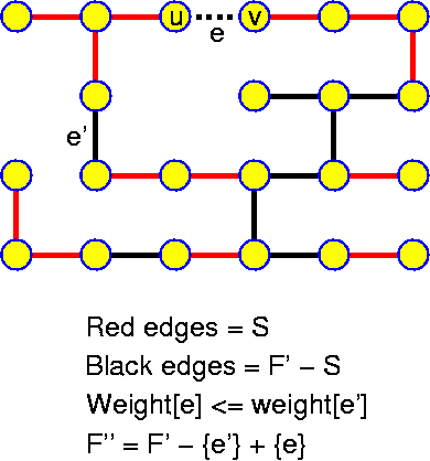
We work out a few details. Assume that edges are objects with two instance variables called u and v, respectively. Also assume that the sorted set of edges is available in an array of edges. Then, one can perform the following steps for the main part of the algorithm:
   for (int i = 0; i < m; i++)
     selected[i] = 0;
   for (int i = 0; i < m; i++) {
     x = find(edges[i].u);
     y = find(edges[i].v);
     if (x != y) {
       selected[i] = 1;
       union(x, y); } }
So, we are performing 2 * m finds and at most n - 1 unions (because there is one union for every edge of the forest and the forest has at most n - 1 edges). We know that the union-find datastructure can be implemented very well: it takes hardly more than linear time. Hence, this time only dominates the overall time consumption when the sorting can be performed in linear time.
Divide and conquer does not appear to make sense for making change. How about greedy? That is,
  void Greedy_Amount_Paying(int current amount) {
  Let current denomination be the highest denomination;
  while (remaining amount to pay != 0) {
    while (current denomination <= remaining amount) {
      pay a coin of current denomination;
      remaining amount -= current denomination; }
    current denomination = next smaller denomination; } }
Because there are coins of denomination 1, this algorithm will always be able to pay the required amount. It is efficient: if the algorithm composes a pile of c coins, then the algorithm takes O(n + c) time, which might be the optimal. The algorithm requires (apart from the output) only O(1) memory. The remaining question is about the quality. Is the number of used couns minimum? A rigorous proof can be given using induction for each factor of 10. We only check the base case that all amounts below 10 are treated optimally. For numbers up to 10 it is easy to check that --, 1, 2, 2 + 1, 2 + 2, 5, 5 + 1, 5 + 2, 5 + 2 + 1, 5 + 2 + 2 are the best possible decompositions.
For most optimization problems one can easily formulate a greedy algorithm. Though they are easy and fast, they are not always leading to the maximum/minimum value of the objective function. In this context it is quite conventional to call the solution of a greedy algorithm optimAL and not optimUM and the values maximAL/minimAL instead of maximUM/minimUM. value.
The greedy algorithms are all trivial from the algorithmic point of view. The only issue is how to repeatedly find the lightest/heaviest remaining object that was not considered before. One option is to first sort all objects according to the cost function (assuming it is not changing over time), the alternative is to insert all elements in a priority queue (which can be created in O(n) time for n objects), and then to repeatedly extract the minimum/maximum element. In the case of the spanning forests, this latter approach might be better if there are many edges: as soon as we have a single tree, we can stop. (A more clever variant first runs the priority queue algorithm for a number of edges, then throws away all the edges running within the same component, and then sorting the surviving edges.) More interesting is mostly the proof that the solution is actually optimUM.
The basic idea of divide-and-conquer algorithms (but people like this name very much and glue it on any algorithm that has a similar structure) are the following three steps:
In the case of quick sort, the division was quite hard, while the recombination only consists of concatenating the answers in the right order. In the integer multiplication, we had three subproblems, and the recombination phase consists of the final shifting, adding and subtracting.
(n over k) = (n - 1 over k - 1) + (n - 1 over k), for all k with 0 < k < n.(n over 0) = (n over n) = 1 and all other values are 0.
This immediately suggests a recursive algorithm, the only operation used is addition, so this appears nice. However, the time consumption becomes terrible: if we use N = n + k, then we see that T(N) = T(N - 1) + T(N - 2) + something. This we have seen before!
Just as one should not compute Fibonacci numbers top-down recursively, so should one not compute binomial coefficients recursively. But, of course, just as Fibonacci numbers could also be computed in a bottom-up fashion, so can one do this here just compute the entries of Pascal's triangle row by row, always saving the last row.
Doing this, the whole computation takes Theta(n * k) time and Theta(k) space, which is clearly much better than the recursive algorithm. An important advantage over the conventional multiplicative way of computing binomial coefficients as n! / (k! * (n - k)!) is that all involved numbers are relatively small.
In the case of the binomial coefficients, this gives at least some saving, though it is hard to estimate how much. In many other cases it is clear that most of al the possible values for smaller problems are not needed, so it would be wastefull to compute al of them. At the same time it may be hard to tell explicitly which values must be computed to find the answer for the whole problem. The top-down aproach with a table works fine for such cases.
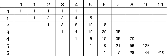
This argument has one flaw: how can we test whether an entry is already computed or not? Only by checking some flag. For example, one might initially write a value that cannot possibly be a correct answer, 0 would do if we know that all real values are positive. However, the memory might contain values that appear reasonable right from the start (or more often: from an earlier call to the same routine with different values). So, we must intiallize the whole space, which takes all the time we wanted to save. What can we do about this?
In the first place: setting positions to 0 goes considerably faster than computing a value, so practically this may be a big improvement even though theoretically it is all the same.
In the second place, it may hapen that we want to evaluate the function for many values. In that case, it is a very good and practical idea to create a table of sufficient size for the largest problem that will be solved. This table is initialized before the first computation. Then when the computation is performed, we keep track of all the entries that are used in a list (implemented as array). After the routine all these positions are reset. In this way the omputation becomes only marginally slower, avoiding the initialization costs.
Finally there is the idea of virtual initialization, which is not so practical though.
c(N) = 1 + min_{0 <= i < n} {c(N - d_i)}.This says nothing more than that a large sum can be payed optimally by starting to pay that coin that leads to a sum that requires the fewest further coins.
This observation immediately leads to algorithms constructing optimum schedules. It is clearly not a good idea to do this recursively without added cleverness: the time would clearly be exponential, similar to Fibonacci (but even worse). The real way of doing it is, of course, dynamic programming. One can either do this bottom-up or top-down as discussed above. Anyway, this requires something like Theta(n * N) time, which sounds quite bad. Once the table is constructed, this algorithm requires O(n * number of coins) time to actually find the optimum way of paying an amount.
There is an alternative way of finding the schedule. It bases on the observation that it does not matter in which order the coins are payed out. So, for example we can pay the coins in order of decreasing denomination. This is just as in the greedy algorithm, the difference being that the largest coin does not need to be the largest possible coin. Thus, we pay 88 as 40 + 40 + 4 + 4 and not as 4 + 40 + 40 + 4. But the greedy algorithm would pay 60 + 10 + 10 + 6 + 1 + 1. This implies that for every coin we can consider to use the same coin once again or to never use it again. If one defines c[i, N] to be the minimum number of coins for paying an amount N using only the i smallest coins, we get
c(i, N) = min{1 + c(i, N - d_{i - 1}, c(i - 1, N)}how much time does this cost? Even here many values must be computed. In general one cannot conclude anything better than Theta(n * N). Of course, if the system is based on a smaller set of n' denominations multiplied with powers of 10, then because we are considering the denominations in decreasing order, we can be sure that for a denomination x * 10^i, at worst we will consider all N - j * 10^i, for 0 <= j <= N / 10^i. So, in that case, the total number of positions that might have to be evaluated is bounded by n' * N + n' * N / 10 + ... <= 10/9 * n' * N <= 10 * N = O(N). In any case, once the whole table has been computed, this method can find the best way of paying an amount in time O(n + number of coins).
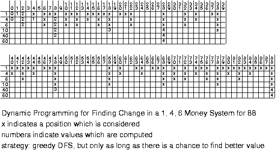
But how if we only have 1 coin of 40? 48 can be payed as 40 + 4 + 4. This is optimal, so N(48) = 3. How many coins do we need for 88? It is no longer true that N(88) = 1 + min{N(28), N(48), N(78), N(82), N(84), N(87)} = 1 + 3 = 4: once we have used the single coin of 40, the best way of paying 48 is as 4 * 10 + 2 * 4, requiring 6 coins.
In general the principal of optimality cannot be applied (without extra care) if there is a "shared resource". Such a shared resource can be found also in the following problem: "Find the longest simple path from node u to node v in a graph". Here a simple path is a path visiting any node only once. Clearly, this problem cannot be split-up: Solving a subproblem does not take into account that one is not allowed to visit the nodes that are visited in the other subproblem.
The space of partial solutions is represented as a graph. The nodes are situations, and the edges link together situations that are one step away. Typically the graph is very large or even infinite, and is not completely constructed at the beginning, but only as far as needed: when the search reaches a k-promising situation (v_0, ..., v_{k - 1}), the algorithm generates the adjacent k + 1 vectors (v_0, ..., v_{k - 1}, v_k). The graph is thus not explicit but implicit.
Backtracking is a method for searching such large implicit graphs. It tries to minimize unnecessary work by never proceeding a path from a node that corresponds to a vector which is not promising.
  procedure backTrack(int k, int* v) {
    /* v is a k-promising vector */
    if (v is a solution)
      printVector(v);
    /* If we only want to find one solution, we can stop here.
       If the extension of a solution never leads to a further
       solution, the following for loop can be skipped. */
    for (each (k + 1)-vector w = (v_0, ..., v_{k - 1}, v_k))
      if (w is (k + 1)-promising)
        backTrack(k + 1, w);
Depending on the problem the tests and the graph are different. The definition of k-promising may also include extra conditions, to guide the search, for example to prevent that equivalent vectors are considered more than once.
The presented backtracking algorithm will explore the graph in a depth-first manner, as this is exactly what recursion gives us. In the following two examples, it does not matter in what order the graph is traversed, so there we can apply DFS, given that this is what one gets easiest. However, there are problems for which even nodes at very large recursion depth may be feasible. If we perform DFS for such problems, it may take unnecessarily long (infinitely) to return from a branch without solutions. In that case one might prefer an alternative graph traversal such as BFS. An even more subtle strategy is to use a priority queue instead of a simple stack or queue, the goal being to more rapidly find really good solutions.
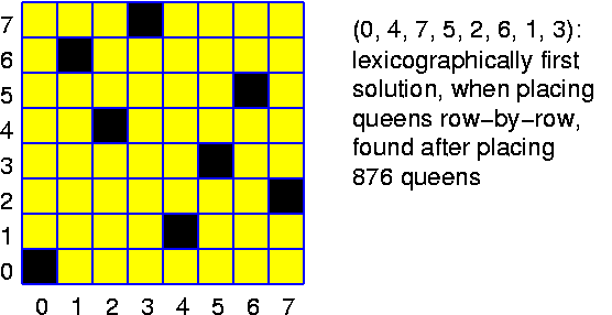
The most dumb idea is to try all subsets of size n. This implies testing (n^2 over n) ~= n^n possibilities, quite outrageous already for k = 8.
Slightly better is to realize that queens should be in different columns. So, a solution is given by a vector (v_0, ..., v_{n - 1}) n which v_i indicates the column in which the queen in row i is positioned. If we now also realize that all v_i must be different, then the number of tests is reduced to n! ~= (n / e)^n. Substantially better, but still not good at all.
A shortcoming of these methods is that we first generate a complete solution, and then test whether it is feasible. Many solutions with a common impossible prefix are generated and tested. Here backtraking comes in and brings large savings (which are very hard to quantify other than by experiment). The program might look as follows. It is called with k == 0.
  void queenPlacement(int k, int n, int position[n]) {
    int i, j;
    boolean column[n];
    boolean main_diag[2 * n - 1];
    boolean anti_diag[2 * n - 1];
    if (k == n)
      printVector(n, position);
    else {

      /* Marking the occupied columns */
      for (j = 0; j < n; j++)
        column[j] = 1;
      for (i = 0; i < k; i++)
        column[position[i]] = 0;

      /* Marking the occupied diagonals */
      for (i = 0; i < 2 * n - 1; i++)
        main_diag[i] = 1;
      for (i = 0; i < k; i++)
        main_diag[position[i] - i + n - 1] = 0;

      /* Marking the occupied anti-diagonals */
      for (i = 0; i < 2 * n - 1; i++)
        anti_diag[i] = 1;
      for (i = 0; i < k; i++)
        anti_diag[position[i] + i] = 0;

      /* Try to place a queen in row k and column j */
      for (j = 0; j < n; j++)
        if (column[j] && main_diag[j - k + n - 1] && anti_diag[j + k]) {
          position[k] = i;
          queenPlacement(k + 1, n, position); } } }
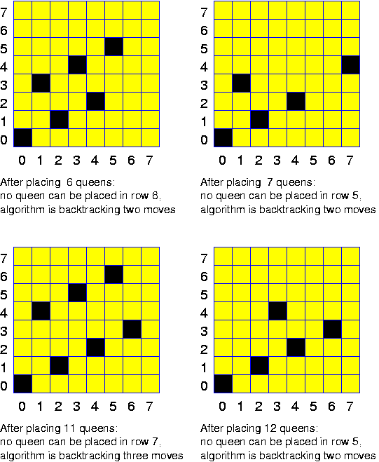
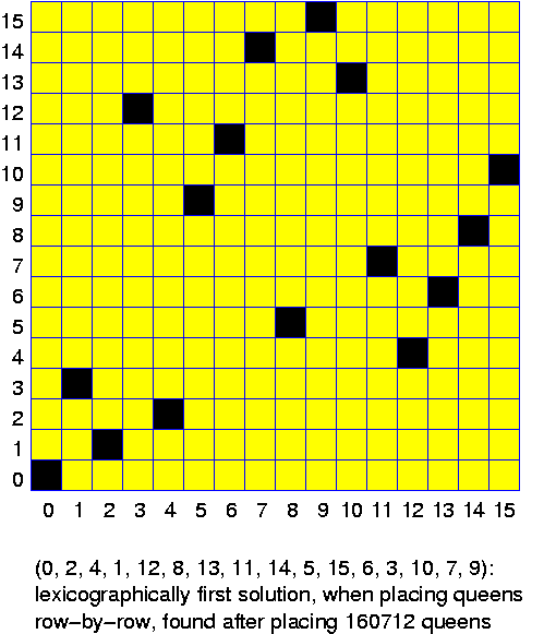
In a real implementation, better performance is achieved by passing even the boolean arrays as arguments. In that case the extra column and diagonals must be added to the sets before the recursion and taken out again after it. It is easy to work these ideas out to obtain a running program in Java.
So, branch-and-bound is in the first place a method to prune the tree corresponding to feasible partial solutions of an optimziation problem. However, in a context of an optimization problem, it is only natural to also try to focus the search on branches that appear most promising. That is, to first develop branches that, based on their lower and upper bounds and other criteria promise to lead to the best solutions. The rational is that developing such branches probably leads to finding improved lower and upper bounds, which allows to prune more of the other branches. Thus, in general one does not perform a pure DFS or BFS search, but rather a tuned search, using a priority queue to maintain the list of generated but not yet completely explored nodes. At every stage we proceed with the node at the head of the priority queue.
Applying branch-and-bound requires specifying at least the following four points:
As soon as you start branching, you are lost!
Problems that can be solved more or less succesfully by the branch-and-bound method are
V = sum_{i = 1}^n x_i * v_i,the task is to maximize V subject to the condition that W' <= W.
W' = sum_{i = 1}^n x_i * w_i,
A greedy solution, maybe the one you intuitively apply yourself when packing for a trip, is to pick the objects in order of decreasing value per weight. This leads to a simple greedy algorithm (compute r_i = v_i / w_i, sort the objects on r_i and add as long as the sum of the selected ones is less than W). Is it good? Yes, it is good, but it is not optimal. If v_1 = 16, v_2 = v_3 = 9, w_1 = 4, w_2 = w_3 = 3 and W = 6, then r_1 = 4, r_2 = r_3 = 3. So, the greedy algorithm would pick the first object and then we cannot take any of the other items. So, V = 16. Taking the other two objects gives V = 18, still respecting W' <= W.
V(x_0, ..., x_{j - 1}) <= sum_{i = 0}^{j - 1} x_i * v_i + (W - sum_{i = 0}^{j - 1} x_i * w_i) * v_j / w_j.The tree is developed in a DFS manner.
We consider again the same example as before. The (w_i, v_i) pairs are (in sorted order): (6, 25), (5, 20), (2, 8), (3, 10), (4, 10), (1, 2). In the following picture the numbers on the left side give lower bounds, the numbers on the right side upper bounds. A normal number along an edge indicates that the packet with this weight is taken in the knapsack, an overlined number indicates that it is not taken. Branches are not pursued when
